KaDE tool paper: supplementary resources.
|
This website provides some supplementary resources about the following paper:
|
KaDE: a tool to compile Kappa rules into (reduced) ODEs models
|
accepted to the tool paper track of CMSB2017. Please cite:
@InProceedings{feret:CMSB2017,
  title = "KaDE: a tool to compile Kappa rules into (reduced) ODEs models",
  booktitle = "Fifteenth International Workshop on Static Analysis and Systems Biology (SASB'17)",
  series = "LNCS/LNBI",
  publisher = "springer",
  volume = "10545",
  note = "to appear, Supplementary information available at \url{www.di.ens.fr/~feret/CMSB2017-tool-paper}",
  author = "Ferdinanda Camporesi and J{\'e}r{\^o}me Feret and Kim Quy{\^e}n L{\'y}"}
Kappa
Software distribution
The nightly build binaries are available here.These versions are without the graphical interface.
It contains binaries for ubuntu, macos, and windows.
Under macOs the binaries are in the zipfile, in the repository Kappapp.app/Contents/Resources/bin.
Sources may be downloaded on the github repository.
git clone https://github.com/Kappa-Dev/KaSim.git
cd KaSim
You need the OCaml native compiler version 4.03.0 or above as well as ocamlbuild, findlib and Yojson library.
To check whether you have them, type
ocamlfind ocamlopt -version
ocamlfind query yojson
If you use a package manager (or opam, the OCaml package manager), OCaml compilers, ocamlbuild and findlib are really likely provided by it. For instance, you may use the following instruction under opam:
opam install ocamlbuild ocamlfind yojsonOtherwise, OCaml native compilers can be downloaded on INRIA's website. The Windows bundle contains ocamlbuild and findlib. Findlib sources are available on camlcity.org . Ocamlbuild is on github.
If you don't have any easier way to install it (opam, apt, rpm, cygwin, ...), Yojson sources are available here (Note that you'll need to compile and install also its dependencies (cppo, easy-format, biniou) from the same website).
To create binaries, simply type:
make allThe compilation of the graphical interface requires Tk and labltk. Instructions to install Tk may be found here.
If you are using opam, labltk may be installed this way:
opam install labltkOnce you have labltk, compile with the option USE_TK=1:
make clean
make USE_TK=1
If compiled, the gui may be launched by using the following instruction (without any command line option):
./KaDEIn the following we recommend to make symbolic links into a repository in your path. For instance, assuming that KaSim repository is directly in your home, and that the repository local/bin is in your path, the following instructions:
cd ..
ln -sf ~/KaSim/bin/* ~/local/bin/
will create the links. Now you may use KaDE from anywhere:
KaDE
Kappa handbook
Kappa handbook may be found here.Other softwares
BioNetGen
BioNetGen distribution may be found here. BNG2.pl is written in the Perl language, version 5.8 or above is required. Most of the Mac OS, linux machines, and windows machine under Cigwin, have to be installed.Erode
ERODE distribution may be found here. ERODE requires Java 8. If ERODE starts, shows the LOGO, and then nothing happen. This is very likely that you do not have Java 8 properly installed. Under MacOS, Oracle may fail in binding appropriately Java. In that case, the installation will report a succes, but the new version will not be usable. MacPort may be a good alternative to install Java and bind it correctly.CellDesigner
CellDesigner distribution may be found here. KaDE SBML output is compatible with CellDesigner. CellDesigner offers tools to visualize and simulate reaction networks.SBML2LaTeX
SBML2LaTeX distribution may be found here. KaDE SBML output is compatible with SBML2LaTeX. SBML2LaTeX translates SBML files into LaTeX.Examples of the paper
Small tutorial
We describe a case study.We consider the following rules :


We denote as γ1, γ2, and γ3 the corrected rate constants of these rules. With the so-called Biochemist convention, which roughly speaking consists in dividing rates per the number of automorphisms on the left hand side of rules, that are preserved on the right hand side, we have :
- γ1 =
 ;
;
- γ2 =
 ;
;
- γ3 = k3.
Indeed, the third rule makes a difference among the two agents. The non trivial automorphism on the left hand side is not preserved on the right hand side.
Rules 1 and 2 have two automorphisms, whereas rule 3 has only one. As a consequence, the rules are symmetric
with respect to both sites if and only 2 ⋅ = 2 ⋅
= 2 ⋅ = k3, that is to say k1 = k2 = k3.
The model is encoded in Kappa in the following file. The code is given as follows:
2
3 %agent: A(x,y)
4
5 %init: 100 A()
6
7 %var: ’k’ 1
8 %obs: ’asym’ |A(x!1),A(y!1)|
9
10 A(x,y),A(x,y) -> A(x!1,y),A(x!1,y) @’k’
11 A(x,y),A(x,y) -> A(x!1,y),A(x,y!1) @’k’
12 A(x,y),A(x,y) -> A(x,y!1),A(x,y!1) @’k’
13
14 #We use the third convention (consider only the automorphisms in the lhs
15 # that are preserved in the rhs). There are two of them in the first and
16 # in the third rule. Only one in the second one. Hence the rate of the first
18 # and third aredivided by 2.
Line 3 defines the signature of the agent A, and line 5 defines its initial concentration. Line 7 defines a parameter. Any further model reduction remain valid if we change this parameter. Line 8 defines the observable : the concentration of asymmetric dimers will be tracked during the simulation. Lines from 10 to 12 define the rules of the model. Their constant rate is set to k, which is considered as an uninterpreted variable.
We use the following command line to generate the ODE semantics in OCTAVE :
KaDE --rule-rate-convention Biochemist sym.ka
By default, equivalent sites are not analysed and the OCTAVE backend is used.
The result dumped in the following file.
Integration parameters are given from line 19 to line 26.
20 tend=1;
21 initialstep=1e-05;
22 maxstep=0.02;
23 reltol=0.001;
24 abstol=0.001;
25 period=0.01;
26 nonnegative=false;
We notice at line 29:
that the ODEs has 5 variables : 4 for each kind of biomolecular species and 1 for time advance.
Initial state is defined from line 173 to line
174
175 global nodevar
176 global init
177 Init=zeros(nodevar,1);
178
179 Init(1) = init(1); % A(x, y)
180 Init(2) = init(2); % A(x!1, y), A(x!1, y)
181 Init(3) = init(3); % A(x!1, y), A(x, y!1)
182 Init(4) = init(4); % A(x, y!1), A(x, y!1)
183 Init(5) = init(5); % t
184 end
At line 183 we notice that a special variable is introduced for time. Then, each instruction is annotated with some information referring to the Kappa file. Variables are annotated by the corresponding name in the Kappa file. Initial species are annotated by Kappa expression describing the corresponding bio-molecular species.
The ODEs are given from line 204 to line 228:
205
206 % rule : A(x,y), A(x,y) -> A(x,y!1), A(x,y!1)
207 % reaction: A(x, y) + A(x, y) -> A(x, y!1), A(x, y!1)
208
209 dydt(1)=dydt(1)-1/2*k(3)*y(1)*y(1);
210 dydt(1)=dydt(1)-1/2*k(3)*y(1)*y(1);
211 dydt(4)=dydt(4)+2/2*k(3)*y(1)*y(1);
212
213 % rule : A(x,y), A(x,y) -> A(x!1,y), A(x,y!1)
214 % reaction: A(x, y) + A(x, y) -> A(x!1, y), A(x, y!1)
215
216 dydt(1)=dydt(1)-k(2)*y(1)*y(1);
217 dydt(1)=dydt(1)-k(2)*y(1)*y(1);
218 dydt(3)=dydt(3)+k(2)*y(1)*y(1);
219
220 % rule : A(x,y), A(x,y) -> A(x!1,y), A(x!1,y)
221 % reaction: A(x, y) + A(x, y) -> A(x!1, y), A(x!1, y)
222
223 dydt(1)=dydt(1)-1/2*k(1)*y(1)*y(1);
224 dydt(1)=dydt(1)-1/2*k(1)*y(1)*y(1);
225 dydt(2)=dydt(2)+2/2*k(1)*y(1)*y(1);
226 dydt(5)=1;
227
228 end
Each contribution is annotated with the corresponding reaction and the underlying Kappa rule. The Jacobian of the ODEs is given from line 231 to line 288:
232
233 global nodevar
234 global max_stoc_coef
235 global jacvar
236 global var
237 global k
238 global kd
239 global kun
240 global kdun
241 global stoc
242
243 global jack
244 global jackd
245 global jackun
246 global jackund
247 global jacstoc
248
249 var(2)=y(3); % asym
250
251 k(1)=var(1);
252 k(2)=var(1);
253 k(3)=var(1);
254 jacvar(2,3)=1;
255
256
257 jac=sparse(nodevar,nodevar);
258
259 % rule : A(x,y), A(x,y) -> A(x,y!1), A(x,y!1)
260 % reaction: A(x, y) + A(x, y) -> A(x, y!1), A(x, y!1)
261
262 jac(1,1)=jac(1,1)-1/2*k(3)*y(1);
263 jac(1,1)=jac(1,1)-1/2*k(3)*y(1);
264 jac(1,1)=jac(1,1)-1/2*k(3)*y(1);
265 jac(1,1)=jac(1,1)-1/2*k(3)*y(1);
266 jac(4,1)=jac(4,1)+2/2*k(3)*y(1);
267 jac(4,1)=jac(4,1)+2/2*k(3)*y(1);
268
269 % rule : A(x,y), A(x,y) -> A(x!1,y), A(x,y!1)
270 % reaction: A(x, y) + A(x, y) -> A(x!1, y), A(x, y!1)
271
272 jac(1,1)=jac(1,1)-k(2)*y(1);
273 jac(1,1)=jac(1,1)-k(2)*y(1);
274 jac(1,1)=jac(1,1)-k(2)*y(1);
275 jac(1,1)=jac(1,1)-k(2)*y(1);
276 jac(3,1)=jac(3,1)+k(2)*y(1);
277 jac(3,1)=jac(3,1)+k(2)*y(1);
278
279 % rule : A(x,y), A(x,y) -> A(x!1,y), A(x!1,y)
280 % reaction: A(x, y) + A(x, y) -> A(x!1, y), A(x!1, y)
281
282 jac(1,1)=jac(1,1)-1/2*k(1)*y(1);
283 jac(1,1)=jac(1,1)-1/2*k(1)*y(1);
284 jac(1,1)=jac(1,1)-1/2*k(1)*y(1);
285 jac(1,1)=jac(1,1)-1/2*k(1)*y(1);
286 jac(2,1)=jac(2,1)+2/2*k(1)*y(1);
287 jac(2,1)=jac(2,1)+2/2*k(1)*y(1);
288 end
The definition of the observables are defined from line 297 to line 301:
We now wonder whether the sites are equivalent or not. We use the following command line:
KaDE --rule-rate-convention Biochemist sym.ka --show-symmetries
The status of equivalent sites is described in the log:
Symmetries:
In rules:
************
Agent: A
-Equivalence classes of sites for bindings states:
{x,y}
-Equivalence classes of sites (both):
{x,y}
************
In rules and initial states:
************
Agent: A
-Equivalence classes of sites for bindings states:
{x,y}
-Equivalence classes of sites (both):
{x,y}
************
In rules and algebraic expression:
************
The set of rules and the initial state are symmetric with respect to the pair of sites. This is not the case of the observable. Thus, only backward bisimulation may be used to reduce the system. Indeed, if we ignore the difference between sites x and y, we can no longer express the concentration of the sites x that are free. This excludes forward bisimulation. Backward bisimulations may still be used since the concentration of each species can be computed by from the overall concentration of its equivalence class, since the concentration of two equivalent species are always inversely proportional to their number of automorphisms.
KaDE --rule-rate-convention Biochemist sym.ka --with-symmetries Forward --output ode_with_fwd_sym --output-plot data_fwd.csv
give this octave file. There is indeed no reduction. This is because we observe the concentration of asymetric dimers (where a site x is bound to a site y). Forward bisimulation would ignore the difference between symmetric and asymmetric dimers.
KaDE --rule-rate-convention Biochemist sym.ka --with-symmetries Backward --output ode_with_bwd_sym --output-plot data_bwd.csv
reduces the system by ignoring the difference between sites x and y. This is done by replacing in each product of reaction, every species by an arbitrary representative of its equivalence class, and in each algebraic expression, each species concentration by the product between the concentration of its representative and the relative weight of this species in its equivalence class (which is constant and inversely proportional to its number of automorphisms.)
The OCTAVE output is this file. We notice at line 29, that only three variables remain:
The meaning of these variables is given from line 173 to line 182:
174
175 global nodevar
176 global init
177 Init=zeros(nodevar,1);
178
179 Init(1) = init(1); % A(x, y)
180 Init(2) = init(2); % A(x, y!1), A(x, y!1)
181 Init(3) = init(3); % t
182 end
Thus, there is one variable for time advance, one for free As, and one for dimers. The three kinds of dimers are gathered into a single equivalence class (no matter which sites are bound). KaDE has gathered the three kinds of dimers into a single equivalence class (no matter with sites are bound). For instance, from line to line :
212 % reaction: A(x, y) + A(x, y) -> A(x, y!1), A(x, y!1)
the production of an asymmetric dimer, is replaced with the production of a dimer in which the bond is on both sites y.
The definition of observables is given from line to line :
290
291 global nobs
292 global var
293 obs=zeros(nobs,1);
294
295 t = y(3);
296 var(2)=y(2)/4; % asym
297
298 obs(1)=t; % [T]
299 obs(2)=var(2); % asym
300
301 end
We are interested in asymetric dimers only. We notice that their concentration is obtained by dividing the overall quantity of dimers by . To understand why, we shall have a closer look at the meaning of each variable. There exist two conventions. One variable may denote the number of occurrences of a bio-molecular species, or the number of embeddings between this bio-molecular species and the current state of the system. Both conventions are related by the fact, that the number of embeddings is equal to the number of occurrences multiplied by the number of automorphisms in the bio-molecular species. The reduction of the model replace each occurrence of a dimer into a dimer made of two proteins bond via their site y.
As indicated at line 15:
the convention is to count in number of embeddings. Thus the total number of dimers is /. Then half of them only is an asymetric dimer, which gives /
SBML2LaTeX may be used to convert the output of KaDE into PDF.
Firstly, we translate the different versions of the models in SBML.
KaDE sym.ka --ode-backend SBML --output network
KaDE sym.ka --ode-backend SBML --output network_fwd --with-symmetries Forward
KaDE sym.ka --ode-backend SBML --output network_bwd --with-symmetries Backward
The following command line:
java -jar
launches the graphical interface of SBML2LaTeX.
We compile the LaTeX files thanks to the following instructions:
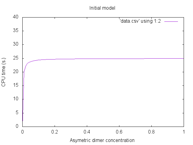
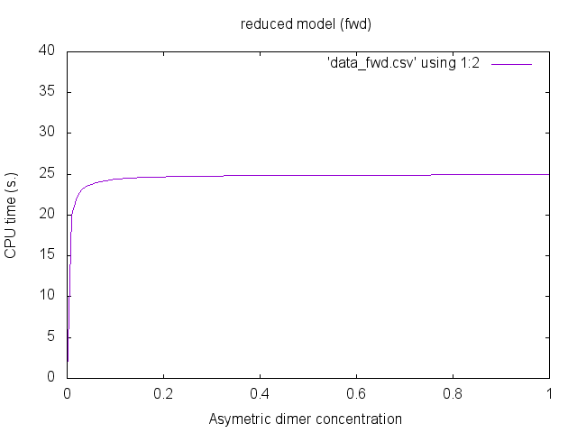
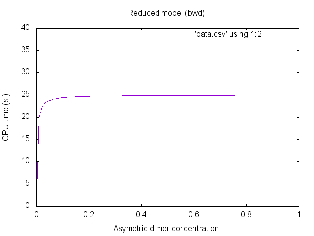
pdflatex network.tex
pdflatex network.tex
pdflatex network_fwd.tex
pdflatex network_fwd.tex
pdflatex network_bwd.tex
pdflatex network_bwd.tex
We obtain the following PDF files: initial model -- reduced model (fwd) -- reduced model (bwd).
Let us check the soundness of our tools, by integrating both ODEs systems.
octave ode.m
octave ode_fwd.m
octave ode_bwd.m
We obtain the three following files: data.csv -- data_fwd.csv -- data_bwd.csv.
We notice that the first two data sets are identical (this is expected since there is no reduction). Additionally, the third data set is almost the same. Despite that the equations have the same solutions, errors due to numerical integration may differ.The concentration of asymetric dimers may be plotted thanks to gnuplot. We use the following gnuplot files: plot.gplot -- plot_fwd.gplot -- plot_bwd.gplot.
gnuplot plot.gplot
gnuplot plot_fwd.gplot
gnuplot plot_bwd.gplot
We obtain the following plots:
Parametric examples
The paper consider three examples, with a parametric size, that we denote by n. We give the Kappa files for each of the three examples with parameter n = 2.
kinase/phosphatase
2 %var: ’kKS’ 0.01
3 %var: ’kdKS’ 1.
4 %var: ’kpS’ 0.1
5 %var: ’kPS’ 0.001
6 %var: ’kdPS’ 0.1
7 %var: ’kuS’ 0.01
8 %agent: K(s)
9 %agent: P(s)
10 %agent: S(x1~u~p,x2~u~p)
11
12 %init: ’Stot’ K(s)
13 %init: ’Stot’ P(s)
14 %init: ’Stot’ S(x1~u,x2~u)
15
16
17 K(s) , S(x1~u) <-> K(s!1) , S(x1~u!1) @ ’kKS’,’kdKS’
18 K(s!1) , S(x1~u!1) -> K(s) , S(x1~p) @ ’kpS’
19 P(s) , S(x1~p) <-> P(s!1) , S(x1~p!1) @ ’kPS’,’kdPS’
20 P(s!1) , S(x1~p!1) -> P(s) , S(x1~u) @ ’kuS’
21 K(s) , S(x2~u) <-> K(s!1) , S(x2~u!1) @ ’kKS’,’kdKS’
22 K(s!1) , S(x2~u!1) -> K(s) , S(x2~p) @ ’kpS’
23 P(s) , S(x2~p) <-> P(s!1) , S(x2~p!1) @ ’kPS’,’kdPS’
24 P(s!1) , S(x2~p!1) -> P(s) , S(x2~u) @ ’kuS’
multiple phosphorylation sites
2 %var: ’ku1’ 14
3 %var: ’kp1’ 15
4 %var: ’ku2’ 98
5 %var: ’kp2’ 75
6 %var: ’ku3’ 686
7 %agent: A(s1~u~p,s2~u~p)
8
9 %init: 100 A(s1~u,s2~u)
10
11 A(s1~p,s2~u) -> A(s1~p,s2~p) @’kp1’
12 A(s1~p,s2~u) -> A(s1~u,s2~u) @’ku1’
13
14
15 A(s1~p,s2~p) -> A(s1~p,s2~u) @’ku2’
16 A(s1~p,s2~p) -> A(s1~u,s2~p) @’ku2’
17
18
19 A(s1~u,s2~u) -> A(s1~u,s2~p) @’kp0’
20 A(s1~u,s2~u) -> A(s1~p,s2~u) @’kp0’
21
22
23 A(s1~u,s2~p) -> A(s1~u,s2~u) @’ku1’
24 A(s1~u,s2~p) -> A(s1~p,s2~p) @’kp1’
multiple phosphorylation sites with counter
2 %var: ’ku1’ 14
3 %var: ’kp1’ 15
4 %var: ’ku2’ 98
5 %agent: A(s1~u~p,s2~u~p,p)
6 %agent: P(l,r)
7
8 %init: 100 A(p!1) , P(l!1,r)
9
10
11
12
13 A(s1~u,p!1) , P(l!1,r) -> A(s1~p,p!1) , P(l!2,r) , P(l!1,r!2) @kp0
14 A(s2~u,p!1) , P(l!1,r) -> A(s2~p,p!1) , P(l!2,r) , P(l!1,r!2) @kp0
15 A(s1~u,p!1) , P(l!1,r!2) , P(l!2,r) -> A(s1~p,p!1) , P(l!2,r!3) , P(l!3,r) , P(l!1,r!2) @kp1
16 A(s1~p,p!1) , P(l!2,r) , P(l!1,r!2) -> A(s1~u,p!1) , P(l!1,r) @ku1
17 A(s2~u,p!1) , P(l!1,r!2) , P(l!2,r) -> A(s2~p,p!1) , P(l!2,r!3) , P(l!3,r) , P(l!1,r!2) @kp1
18 A(s2~p,p!1) , P(l!2,r) , P(l!1,r!2) -> A(s2~u,p!1) , P(l!1,r) @ku1
19 A(s1~p,p!1) , P(l!2,r!3) , P(l!3,r) , P(l!1,r!2) -> A(s1~u,p!1) , P(l!1,r!2) , P(l!2,r) @ku2
20 A(s2~p,p!1) , P(l!2,r!3) , P(l!3,r) , P(l!1,r!2) -> A(s2~u,p!1) , P(l!1,r!2) , P(l!2,r) @ku2
All the files for the description of the models, both in Kappa and in BNGL may be found in this tarball.
All the files, including both the input models and the reduced ones, may be found in this tarball.
kinase/phosphatase
Building Kappa and BNGL models
Here is an OCaml source code to generate the model.
The following instructions:
ocamlopt.opt kinase_phosphatase.ml  -o kinase_phosphatase
mkdir generated_models
mkdir generated_models/kin_phos
./kinase_phosphatase 1 10
will generate the models, in the repository generated_models/kin_phos, in Kappa and in BNG for the parameter n ranging from 1 to 10.
ls generated_models/kin_phos
The Kappa model matches with the BNGL model with distinct sites.
Tarball
The following tarball contains all the input/output files for this model.Input/output files
Each file is available individually in the following table:| n | Kappa file | KaDE (ground system) | KaDE (forward bisimulation) | KaDE (backward bisimulation | BNGL file (with distinct sites) | Network | BNGL file (with multiple sites) | Network |
|---|---|---|---|---|---|---|---|---|
| 1 | Kappa | DotNet | DotNet | DotNet | BNGL | DotNet | BNGL | DotNet |
| 2 | Kappa | DotNet | DotNet | DotNet | BNGL | DotNet | BNGL | DotNet |
| 3 | Kappa | DotNet | DotNet | DotNet | BNGL | DotNet | BNGL | DotNet |
| 4 | Kappa | DotNet | DotNet | DotNet | BNGL | DotNet | BNGL | DotNet |
| 5 | Kappa | DotNet | DotNet | DotNet | BNGL | DotNet | BNGL | DotNet |
| 6 | Kappa | DotNet | DotNet | DotNet | BNGL | DotNet | BNGL | DotNet |
| 7 | Kappa | DotNet | DotNet | DotNet | BNGL | DotNet | BNGL | DotNet |
| 8 | Kappa | DotNet | DotNet | DotNet | BNGL | BNGL | DotNet | |
| 9 | Kappa | DotNet | DotNet | DotNet | BNGL | BNGL | DotNet | |
| 10 | Kappa | DotNet | DotNet | DotNet | BNGL | BNGL | DotNet |
Benchmarks
We obtain the following benchmarks: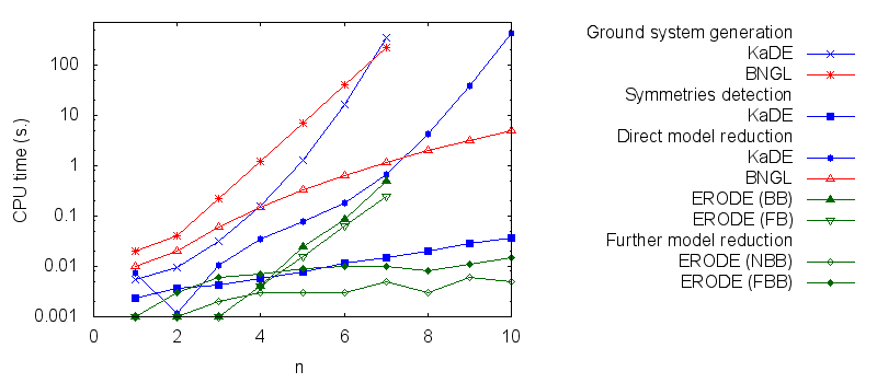
| n | KaDE_wo_sym | KaSa | KaDE_fwd | KaDE_bwd | bngl | bngl_sym | erode_initial (FB) | erode_initial (NFB) | erode_initial (BB) | erode_initial (NBB) | erode_reduced (FB) | erode_reduced (NFB) | erode_reduced (BB) | erode_reduced (NBB) |
|---|---|---|---|---|---|---|---|---|---|---|---|---|---|---|
| 1 | 0.00542 | 0.002386 | 0.007474 | 0.004767 | 0.02 | 0.01 | 0.001 | 0.001 | 0.001 | 0.001 | 0.001 | 0.001 | 0.001 | 0.001 |
| 2 | 0.009713 | 0.003688 | 0.0011809 | 0.010309 | 0.04 | 0.02 | 0.001 | 0.001 | 0.001 | 0.001 | 0.001 | 0.003 | 0.001 | 0.001 |
| 3 | 0.03105 | 0.004322 | 0.010267 | 0.016402 | 0.22 | 0.06 | 0.001 | 0.001 | 0.001 | 0.001 | 0.001 | 0.006 | 0.002 | 0.002 |
| 4 | 0.159678 | 0.005659 | 0.035457 | 0.039075 | 1.23 | 0.15 | 0.004 | 0.008 | 0.004 | 0.005 | 0.002 | 0.007 | 0.003 | 0.003 |
| 5 | 1.26683 | 0.007863 | 0.079153 | 0.084271 | 7.06 | 0.33 | 0.016 | 0.042 | 0.024 | 0.025 | 0.003 | 0.009 | 0.004 | 0.003 |
| 6 | 16.1219 | 0.011796 | 0.183597 | 0.201491 | 39.71 | 0.63 | 0.063 | 0.156 | 0.088 | 0.085 | 0.005 | 0.010 | 0.004 | 0.003 |
| 7 | 344.108 | 0.014771 | 0.677966 | 0.672631 | 222.91 | 1.15 | 0.244 | 0.800 | 0.499 | 0.463 | 0.005 | 0.010 | 0.005 | 0.005 |
| 8 | ? | 0.020017 | 4.22518 | 4.17969 | ? | 1.97 | ? | ? | ? | ? | 0.006 | 0.008 | 0.006 | 0.003 |
| 9 | ? | 0.028944 | 37.8643 | 38.0085 | ? | 3.17 | ? | ? | ? | ? | 0.005 | 0.011 | 0.007 | 0.006 |
| 10 | ? | 0.036031 | 421.908 | 424.09 | ? | 4.91 | ? | ? | ? | ? | 0.007 | 0.015 | 0.009 | 0.005 |
Each computation has been made with a 10 minutes time-out. Computations have been made on a MacBookPro with a 2.8 GHz Intel Core i7 CPU and a 16 Go 1600 MHz DDR3 memory.
In particular we propose to compare the computation of several pipelines for several functionnalities.
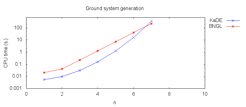
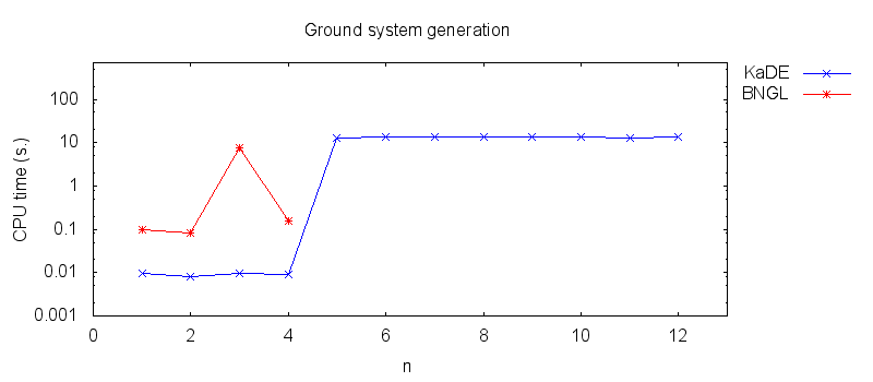
- Firstly, we compare the computation to generate the ground network with BNGL and with KaDE. We obtain the following plots:
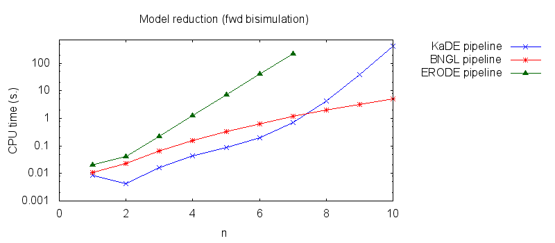
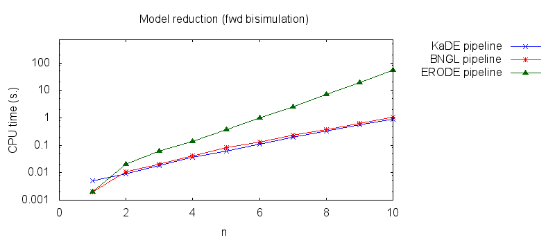
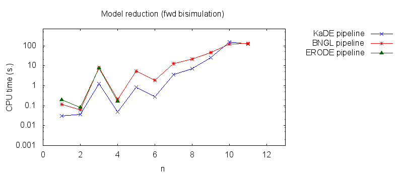
- Secondly, we compare the computation to generate the network reduced by forward bisimulation. In the first pipeline, we use KaDE to generate a reduced network, then we use ERODE to prove the optimality of the reduction (using the algorithm NFB). In the second pipeline, we specify explicitely in the BNGL model, which sites are equivalent, we use BNGL to generate the reduced model, and then we use ERODE to prove the optimality. In the third pipeline, we use BNGL to generate the ground network, and then we use ERODE to reduce this network by the means of forward bisimulation (using the faster, but potentially incomplete, algorithm FB).
It is worth stressing out that equivalent sites are infered automatically by KaDE and ERODE, whereas they have to be specified explicitly by the end-used in BNGL. ERODE can also go further by inferring the coarsest bisimulation that is specified by a parition of the set of bio-molecular species.
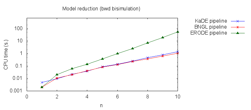
We obtain the following plots: - Thirdly, we compare the computation to generate the network reduced by backward bisimulation. In the first pipeline, we use KaDE to generate a reduced network, then we use ERODE to prove the optimality of the reduction (using the algorithm NBB). In the second pipeline, we specify explicitely in the BNGL model, which sites are equivalent, we use BNGL to generate the reduced model, and then we use ERODE to search for further potential reduction (since ERODE focuses on uniform bisimulation, it cannot prove the optimality of the reduction). In the third pipeline, we use BNGL to generate the ground network, and then we use ERODE to reduce this network by the means of backward bisimulation (using the faster, but potentially incomplete, algorithm BB).
It is worth stressing out that equivalent sites are infered automatically by KaDE and ERODE, whereas they have to be specified explicitly by the end-used in BNGL.
We obtain the following plots:

multi-phosphorilation sites
Building Kappa and BNGL models
Here is an OCaml source code to generate the model.
The following instructions:
ocamlopt.opt kinase_phosphatase.ml  -o kinase_phosphatase
mkdir generated_models
mkdir generated_models/kin_phos
./multi_phos 1 10
will generate the models, in the repository generated_models/multi_phos, in Kappa and in BNG for the parameter n ranging from 1 to 10.
ls generated_models/multi_phos
The Kappa model matches with the BNGL model with distinct sites.
Tarball
The following tarball contains all the input/output files for this model.Input/output files
Each file is available individually in the following table:| n | Kappa file | KaDE (ground system) | KaDE (forward bisimulation) | KaDE (backward bisimulation | BNGL file (with distinct sites) | Network | BNGL file (with multiple sites) | Network |
|---|---|---|---|---|---|---|---|---|
| 1 | Kappa | DotNet | DotNet | DotNet | BNGL | DotNet | BNGL | DotNet |
| 2 | Kappa | DotNet | DotNet | DotNet | BNGL | DotNet | BNGL | DotNet |
| 3 | Kappa | DotNet | DotNet | DotNet | BNGL | DotNet | BNGL | DotNet |
| 4 | Kappa | DotNet | DotNet | DotNet | BNGL | DotNet | BNGL | DotNet |
| 5 | Kappa | DotNet | DotNet | DotNet | BNGL | DotNet | BNGL | DotNet |
| 6 | Kappa | DotNet | DotNet | DotNet | BNGL | DotNet | BNGL | DotNet |
| 7 | Kappa | DotNet | DotNet | DotNet | BNGL | DotNet | BNGL | DotNet |
| 8 | Kappa | DotNet | DotNet | DotNet | BNGL | DotNet | BNGL | DotNet |
| 9 | Kappa | DotNet | DotNet | DotNet | BNGL | DotNet | BNGL | |
| 10 | Kappa | DotNet | DotNet | DotNet | BNGL | DotNet | BNGL |
Benchmarks
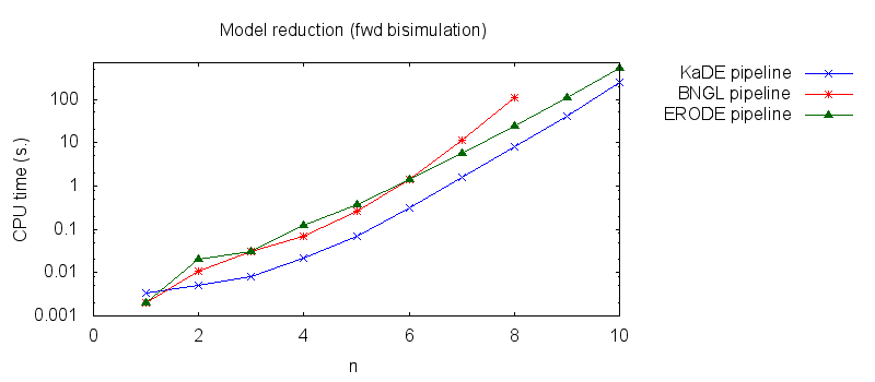
We obtain the following benchmarks: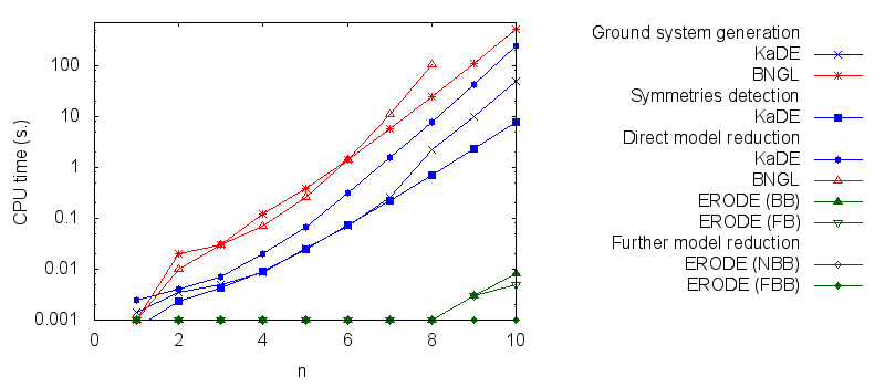
| n | KaDE_wo_sym | KaSa | KaDE_fwd | KaDE_bwd | bngl | bngl_sym | erode_initial (FB) | erode_initial (NFB) | erode_initial (BB) | erode_initial (NBB) | erode_reduced (FB) | erode_reduced (NFB) | erode_reduced (BB) | erode_reduced (NBB) |
|---|---|---|---|---|---|---|---|---|---|---|---|---|---|---|
| 1 | 0.001394 | 0.000722 | 0.002418 | 0.002514 | 0.001 | 0.001 | 0.001 | 0.001 | 0.001 | 0.001 | 0.001 | 0.001 | 0.001 | 0.001 |
| 2 | 0.003474 | 0.002305 | 0.003985 | 0.004139 | 0.02 | 0.01 | 0.001 | 0.001 | 0.001 | 0.001 | 0.001 | 0.001 | 0.001 | 0.001 |
| 3 | 0.004863 | 0.004226 | 0.007032 | 0.007262 | 0.03 | 0.03 | 0.001 | 0.001 | 0.001 | 0.001 | 0.001 | 0.001 | 0.001 | 0.001 |
| 4 | 0.008634 | 0.008914 | 0.020552 | 0.018946 | 0.12 | 0.07 | 0.001 | 0.001 | 0.001 | 0.001 | 0.001 | 0.001 | 0.001 | 0.001 |
| 5 | 0.026137 | 0.025071 | 0.067181 | 0.069171 | 0.38 | 0.26 | 0.001 | 0.001 | 0.001 | 0.001 | 0.001 | 0.001 | 0.001 | 0.001 |
| 6 | 0.069118 | 0.073423 | 0.311556 | 0.33069 | 1.44 | 1.43 | 0.001 | 0.001 | 0.001 | 0.001 | 0.001 | 0.001 | 0.001 | 0.001 |
| 7 | 0.25431 | 0.224123 | 1.57005 | 1.60526 | 5.72 | 11.10 | 0.001 | 0.001 | 0.001 | 0.001 | 0.001 | 0.001 | 0.001 | 0.001 |
| 8 | 2.19546 | 0.708071 | 7.88053 | 7.96044 | 24.52 | 106.26 | 0.001 | 0.001 | 0.001 | 0.001 | 0.001 | 0.001 | 0.001 | 0.001 |
| 9 | 10.1247 | 2.29603 | 41.7526 | 43.3281 | 110.73 | 0.003 | 0.003 | 0.003 | 0.002 | 0.001 | 0.001 | 0.001 | 0.001 | |
| 10 | 48.572 | 7.7361 | 250.509 | 253.594 | 518.90 | 0.005 | 0.007 | 0.008 | 0.008 | 0.001 | 0.001 | 0.001 | 0.001 |
Each computation has been made with a 10 minutes time-out. Computations have been made on a MacBookPro with a 2.8 GHz Intel Core i7 CPU and a 16 Go 1600 MHz DDR3 memory.
In particular we propose to compare the computation of several pipelines for several functionnalities.
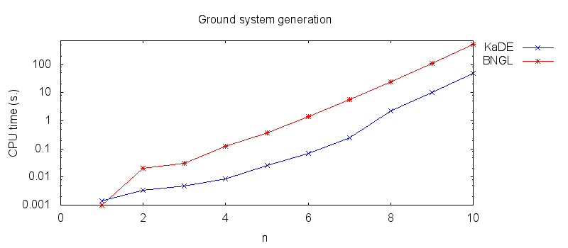
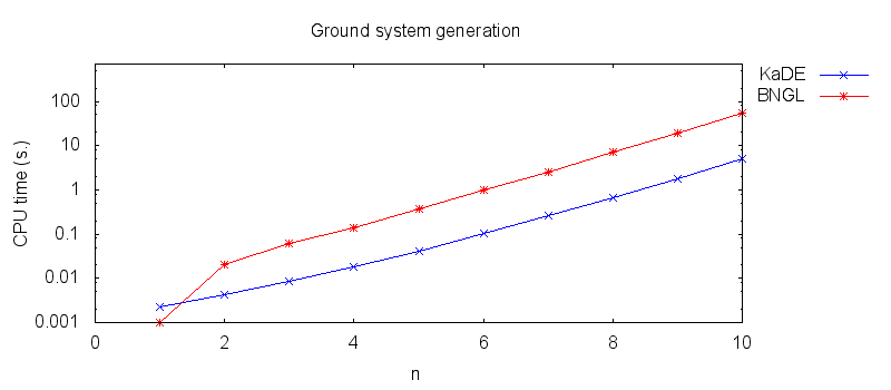
- Firstly, we compare the computation to generate the ground network with BNGL and with KaDE. We obtain the following plots:
- Secondly, we compare the computation to generate the network reduced by forward bisimulation. In the first pipeline, we use KaDE to generate a reduced network, then we use ERODE to prove the optimality of the reduction (using the algorithm NFB). In the second pipeline, we specify explicitely in the BNGL model, which sites are equivalent, we use BNGL to generate the reduced model, and then we use ERODE to prove the optimality. In the third pipeline, we use BNGL to generate the ground network, and then we use ERODE to reduce this network by the means of forward bisimulation (using the faster, but potentially incomplete, algorithm FB).
It is worth stressing out that equivalent sites are infered automatically by KaDE and ERODE, whereas they have to be specified explicitly by the end-used in BNGL. ERODE can also go further by inferring the coarsest bisimulation that is specified by a parition of the set of bio-molecular species.
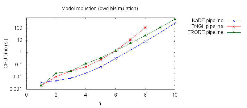
We obtain the following plots: - Thirdly, we compare the computation to generate the network reduced by backward bisimulation. In the first pipeline, we use KaDE to generate a reduced network, then we use ERODE to prove the optimality of the reduction (using the algorithm NBB). In the second pipeline, we specify explicitely in the BNGL model, which sites are equivalent, we use BNGL to generate the reduced model, and then we use ERODE to search for further potential reduction (since ERODE focuses on uniform bisimulation, it cannot prove the optimality of the reduction). In the third pipeline, we use BNGL to generate the ground network, and then we use ERODE to reduce this network by the means of backward bisimulation (using the faster, but potentially incomplete, algorithm BB).
It is worth stressing out that equivalent sites are infered automatically by KaDE and ERODE, whereas they have to be specified explicitly by the end-used in BNGL.
We obtain the following plots:
multi-phosphorilation sites (encoded with explicit counter)
Building Kappa and BNGL models
Here is an OCaml source code to generate the model.
The following instructions:
ocamlopt.opt multi_phos_with_counter.ml  -o multi_phos_with_counter
mkdir generated_models
mkdir generated_models/multi_phos_with_counter
./multi_phos_with_counter 1 10
will generate the models, in the repository generated_models/multi_phos, in Kappa and in BNG for the parameter n ranging from 1 to 10.
ls generated_models/multi_phos_with_counter
The Kappa model matches with the BNGL model with distinct sites.
Tarball
The following tarball contains all the input/output files for this model.Input/output files
Each file is available individually in the following table:| n | Kappa file | KaDE (ground system) | KaDE (forward bisimulation) | KaDE (backward bisimulation | BNGL file (with distinct sites) | Network | BNGL file (with multiple sites) | Network |
|---|---|---|---|---|---|---|---|---|
| 1 | Kappa | DotNet | DotNet | DotNet | BNGL | DotNet | BNGL | DotNet |
| 2 | Kappa | DotNet | DotNet | DotNet | BNGL | DotNet | BNGL | DotNet |
| 3 | Kappa | DotNet | DotNet | DotNet | BNGL | DotNet | BNGL | DotNet |
| 4 | Kappa | DotNet | DotNet | DotNet | BNGL | DotNet | BNGL | DotNet |
| 5 | Kappa | DotNet | DotNet | DotNet | BNGL | DotNet | BNGL | DotNet |
| 6 | Kappa | DotNet | DotNet | DotNet | BNGL | DotNet | BNGL | DotNet |
| 7 | Kappa | DotNet | DotNet | DotNet | BNGL | DotNet | BNGL | DotNet |
| 8 | Kappa | DotNet | DotNet | DotNet | BNGL | DotNet | BNGL | DotNet |
| 9 | Kappa | DotNet | DotNet | DotNet | BNGL | DotNet | BNGL | DotNet |
| 10 | Kappa | DotNet | DotNet | DotNet | BNGL | DotNet | BNGL | DotNet |
Benchmarks
We obtain the following benchmarks: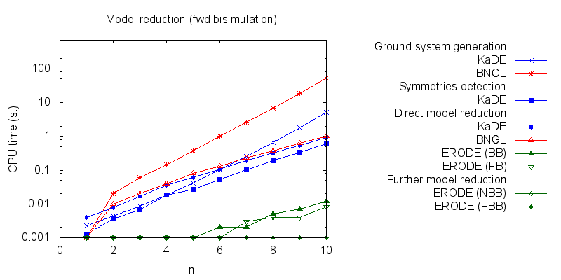
| n | KaDE_wo_sym | KaSa | KaDE_fwd | KaDE_bwd | bngl | bngl_sym | erode_initial (FB) | erode_initial (NFB) | erode_initial (BB) | erode_initial (NBB) | erode_reduced (FB) | erode_reduced (NFB) | erode_reduced (BB) | erode_reduced (NBB) |
|---|---|---|---|---|---|---|---|---|---|---|---|---|---|---|
| 1 | 0.00225 | 0.001286 | 0.004046 | 0.003873 | 0.001 | 0.001 | 0.001 | 0.001 | 0.001 | 0.001 | 0.001 | 0.001 | 0.001 | 0.001 |
| 2 | 0.004318 | 0.003685 | 0.007873 | 0.008793 | 0.02 | 0.01 | 0.001 | 0.001 | 0.001 | 0.001 | 0.001 | 0.001 | 0.001 | 0.001 |
| 3 | 0.008547 | 0.006645 | 0.017025 | 0.020627 | 0.06 | 0.02 | 0.001 | 0.001 | 0.001 | 0.001 | 0.001 | 0.001 | 0.001 | 0.001 |
| 4 | 0.018465 | 0.018465 | 0.036521 | 0.037319 | 0.14 | 0.04 | 0.001 | 0.001 | 0.001 | 0.001 | 0.001 | 0.001 | 0.001 | 0.001 |
| 5 | 0.041986 | 0.026849 | 0.06203 | 0.087131 | 0.37 | 0.08 | 0.001 | 0.002 | 0.001 | 0.001 | 0.001 | 0.001 | 0.001 | 0.001 |
| 6 | 0.101352 | 0.052174 | 0.106849 | 0.138138 | 1.00 | 0.13 | 0.001 | 0.003 | 0.002 | 0.003 | 0.001 | 0.001 | 0.001 | 0.001 |
| 7 | 0.255698 | 0.100566 | 0.191022 | 0.251259 | 2.58 | 0.23 | 0.003 | 0.006 | 0.002 | 0.002 | 0.001 | 0.001 | 0.001 | 0.001 |
| 8 | 0.670282 | 0.194196 | 0.324019 | 0.459048 | 6.96 | 0.37 | 0.004 | 0.004 | 0.005 | 0.005 | 0.001 | 0.001 | 0.001 | 0.001 |
| 9 | 1.76816 | 0.332928 | 0.54416 | 0.791958 | 18.89 | 0.62 | 0.004 | 0.005 | 0.007 | 0.005 | 0.001 | 0.001 | 0.001 | 0.001 |
| 10 | 5.16022 | 0.588872 | 0.899689 | 1.37989 | 54.40 | 1.03 | 0.008 | 0.011 | 0.012 | 0.012 | 0.001 | 0.001 | 0.001 | 0.001 |
Each computation has been made with a 10 minutes time-out. Computations have been made on a MacBookPro with a 2.8 GHz Intel Core i7 CPU and a 16 Go 1600 MHz DDR3 memory.
In particular we propose to compare the computation of several pipelines for several functionnalities.- Firstly, we compare the computation to generate the ground network with BNGL and with KaDE. We obtain the following plots:
- Secondly, we compare the computation to generate the network reduced by forward bisimulation. In the first pipeline, we use KaDE to generate a reduced network, then we use ERODE to prove the optimality of the reduction (using the algorithm NFB). In the second pipeline, we specify explicitely in the BNGL model, which sites are equivalent, we use BNGL to generate the reduced model, and then we use ERODE to prove the optimality. In the third pipeline, we use BNGL to generate the ground network, and then we use ERODE to reduce this network by the means of forward bisimulation (using the faster, but potentially incomplete, algorithm FB).
It is worth stressing out that equivalent sites are infered automatically by KaDE and ERODE, whereas they have to be specified explicitly by the end-used in BNGL. ERODE can also go further by inferring the coarsest bisimulation that is specified by a parition of the set of bio-molecular species.
We obtain the following plots: - Thirdly, we compare the computation to generate the network reduced by backward bisimulation. In the first pipeline, we use KaDE to generate a reduced network, then we use ERODE to prove the optimality of the reduction (using the algorithm NBB). In the second pipeline, we specify explicitely in the BNGL model, which sites are equivalent, we use BNGL to generate the reduced model, and then we use ERODE to search for further potential reduction (since ERODE focuses on uniform bisimulation, it cannot prove the optimality of the reduction). In the third pipeline, we use BNGL to generate the ground network, and then we use ERODE to reduce this network by the means of backward bisimulation (using the faster, but potentially incomplete, algorithm BB).
It is worth stressing out that equivalent sites are infered automatically by KaDE and ERODE, whereas they have to be specified explicitly by the end-used in BNGL.
We obtain the following plots:
Other examples
We have manually translated each model of the BNGL distribution into Kappa. We have used the static analyzer KaSa to check that there is no dead code in models. We found the rule for transphosphorylation of Fyn by SH2-bound Lyn was wrong in each BNGL model, we corrected it as well as in the kappa models.
Remark on equivalent sites
It is worth noticing that the operational semantics on equivalent sites in BNGL does not match with the intuitive encoding with multiple identified sites. Let us consider an example with a protein A with a site x that may take the state u or p and two sites l that may take the state u, p, or q.
We consider the following rule in BNGL:
This means that the site x of a protein A may get the state p at rate k provided that at least one site l is in state u.
An intuitive encoding with identified sites would be the following:
The previous encoding is quantitatively wrong, both rules may be used to activate the site x of a protein A with both sites l1 and l2 in state u, with an overall rate of 2k (instead of k in the BNGL model with equivalent sites).
A correct encoding requires to refine the states of sites l1 and l2:2 A(x~u,l1~u,l2~p) -> A(x~p,l1~u,l2~p) k
3 A(x~u,l1~u,l2~q) -> A(x~p,l1~u,l2~q) k
4 A(x~u,l1~p,l2~u) -> A(x~p,l1~p,l2~u) k
5 A(x~u,l1~q,l2~u) -> A(x~p,l1~q,l2~u) k
This approach can be generalised. Consider a protein with some equivalent sites. Consider a rule that tests some of these sites. For each occurrence of agent and each kind of equivalent sites, the sites of this kind may be partitioned into isomorphic classes (two distinct classes stand for two distinct properties to specify the context of the site). Let us assume that there are n equivalence classes. Then we have to consider every function mapping each of the equivalent sites to a subset of these equivalence classes. The interpretation of each function is that each site matches the context of (or the property denoted by) each equivalence class in its image. Then each function is associated with a set of rules. The rule is obtained by refining the initial ones by enforcing, for each site, the properties to be satisfied (for each equivalence class in the image of the site), and enforcing the negation of the properties that are not (for each equivalence class that is not in the image of the site). Since there is no negation, enforcing the negation of a property requires to cover all the other cases, by a set of mutually incompatible conditions.
Some conditions (positive and/or negative) may not be compatible. Thus, a solver may be used to cut irrealisable refinements on the fly.
Input files
This table contains the examples that are provided in the BNGL repository. For each model, we provide the BNGL file and the Kappa model.
| Id | Example name | BNGL file (with multiples sites) | BNGL file (with distinct sites) | Kappa file | Number of bio-molecular species in the initial model | Number of bio-molecular species in the reduced model | Note/current status |
|---|---|---|---|---|---|---|---|
| 1 | test_continue | BNGL | BNGL | Kappa | 22 | 22 | |
| 2 | Repressilator | BNGL | BNGL | Kappa | 51 | 16 | |
| 3 | egfr_net | BNGL | BNGL | Kappa | 356 | 356 | |
| 4 | egfr_net_red | BNGL | BNGL | Kappa | 40 | 40 | |
| 5 | fceri_ji | BNGL | BNGL | Kappa | 654 | 354 | |
| 6 | fceri_ji_red | BNGL | BNGL | Kappa | 654 | 172 | |
| 7 | fceri_lyn_745 | BNGL | BNGL | Kappa | 1411 | 745 | |
| 8 | fceri_fyn | BNGL | BNGL | Kappa | 2457 | 1281 | Dead rules have been corrected |
| 9 | fceri_fyn_lig | BNGL | BNGL | Kappa | 4858 | 2506 | Dead rules have been corrected |
| 10 | fceri_gamma2 | BNGL | BNGL | Kappa | 6646 | 3786 | |
| 11 | fceri_trimer | BNGL | BNGL | Kappa | time out | 2954 | |
| 12 | fceri_fyn_trimer | BNGL | BNGL | Kappa | time-out | time-out | Dead rules have been corrected |
Benchmarks
We obtain the following benchmarks: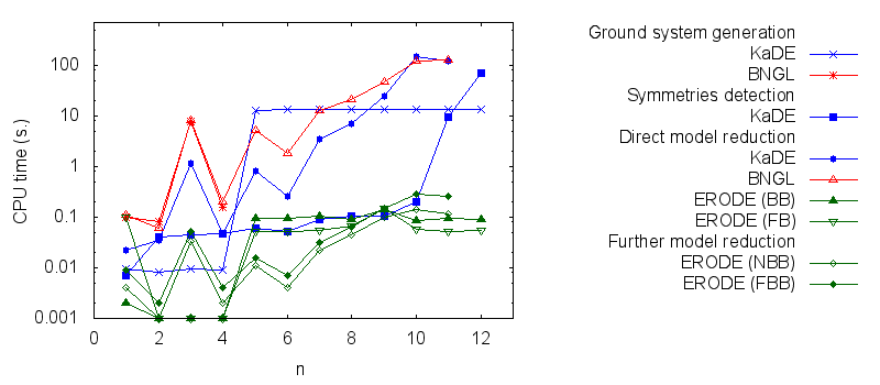
| n | KaDE_wo_sym | KaSa | KaDE_fwd | KaDE_bwd | bngl | bngl_sym | erode_initial (FB) | erode_initial (NFB) | erode_initial (BB) | erode_initial (NBB) | erode_reduced (FB) | erode_reduced (NFB) | erode_reduced (BB) | erode_reduced (NBB) |
|---|---|---|---|---|---|---|---|---|---|---|---|---|---|---|
| 1 | 0.009526 | 0.007193 | 0.02239 | 0.019819 | 0.10 | 0.11 | 0.10 | 0.005 | 0.002 | 0.002 | 0.009 | 0.004 | ||
| 2 | 0.008076 | 0.041444 | 0.034518 | 0.034876 | 0.08 | 0.06 | 0.001 | 0.003 | 0.001 | 0.001 | 0.001 | 0.002 | 0.001 | 0.001 |
| 3 | 0.009402 | 0.045191 | 1.1848 | 1.00853 | 7.68 | 8.22 | 0.001 | 0.001 | 0.001 | 0.001 | 0.053 | 0.033 | ||
| 4 | 0.009039 | 0.047175 | 0.04607 | 0.049943 | 0.16 | 0.20 | 0.001 | 0.001 | 0.001 | 0.001 | 0.001 | 0.004 | 0.002 | 0.002 |
| 5 | 13.0687 | 0.059046 | 0.824042 | 0.834501 | 5.19 | 0.053 | 0.127 | 0.093 | 0.099 | 0.005 | 0.016 | 0.010 | 0.011 | |
| 6 | 13.1851 | 0.05224 | 0.263311 | 0.273658 | 1.85 | 0.052 | 0.134 | 0.094 | 0.095 | 0.002 | 0.007 | 0.002 | 0.004 | |
| 7 | 13.2498 | 0.089625 | 3.48695 | 3.57872 | 13.02 | 0.054 | 0.127 | 0.106 | 0.076 | 0.015 | 0.031 | 0.021 | 0.022 | |
| 8 | 13.1831 | 0.106721 | 6.94145 | 6.9275 | 21.36 | 0.066 | 0.138 | 0.092 | 0.088 | 0.035 | 0.064 | 0.043 | 0.044 | |
| 9 | 13.2876 | 0.107225 | 24.8929 | 24.7812 | 46.48 | 0.149 | 0.212 | 0.141 | 0.119 | 0.074 | 0.149 | 0.096 | 0.102 | |
| 10 | 13.2621 | 0.198361 | 151.554 | 151.188 | 121.18 | 0.058 | 0.133 | 0.088 | 0.103 | 0.104 | 0.284 | 0.148 | 0.145 | |
| 11 | 13.1249 | 9.38133 | 119.584 | 118.768 | 128.35 | 0.051 | 0.135 | 0.093 | 0.094 | 0.051 | 0.259 | 0.117 | 0.115 | |
| 12 | 13.232 | 69.7763 | 0.054 | 0.138 | 0.092 | 0.135 |
Each computation has been made with a 10 minutes time-out. Computations have been made on a MacBookPro with a 2.8 GHz Intel Core i7 CPU and a 16 Go 1600 MHz DDR3 memory.
In particular we propose to compare the computation of several pipelines for several functionnalities.
- Firstly, we compare the computation to generate the ground network with BNGL and with KaDE. We obtain the following plots:
- Secondly, we compare the computation to generate the network reduced by forward bisimulation. In the first pipeline, we use KaDE to generate a reduced network, then we use ERODE to prove the optimality of the reduction. In the second pipeline, we skip the proof of optimality. In the third pipeline, we specify explicitely in the BNGL model, which sites are equivalent, we use BNGL to generate the reduced model, and then we use ERODE to prove the optimality. In the fourth pipeline, we skip the proof of optimality. In the fifth pipeline, we use BNGL to generate the ground network, and then we use ERODE to reduce this network by the means of forward bisimulation.
It is worth stressing out that equivalent sites are infered automatically by KaDE and ERODE, whereas they have to be specified explicitly by the end-used in BNGL. ERODE can also go further by inferring the coarsest bisimulation that is specified by a parition of the set of bio-molecular species.
We obtain the following plots: - Thirdly, we compare the computation to generate the network reduced by backward bisimulation. In the first pipeline, we use KaDE to generate a reduced network, then we use ERODE to prove the optimality of the reduction (using the algorithm NBB). In the second pipeline, we specify explicitely in the BNGL model, which sites are equivalent, we use BNGL to generate the reduced model, and then we use ERODE to search for further potential reduction (since ERODE focuses on uniform bisimulation, it cannot prove the optimality of the reduction). In the third pipeline, we use BNGL to generate the ground network, and then we use ERODE to reduce this network by the means of backward bisimulation (using the faster, but potentially incomplete, algorithm BB).
It is worth stressing out that equivalent sites are infered automatically by KaDE and ERODE, whereas they have to be specified explicitly by the end-used in BNGL.
We obtain the following plots:

References
Tools- Boutillier, P., Feret, J., Krivine, J., Q., Kim Ly: Kasim development homepage, http://kappalanguage.org.
- Cardelli, L., Tribastone, M., Tschaikowski, M., Vandin, A.: ERODE: A tool for the evaluation and reduction of ordinary differential equations. In: Legay, A., Margaria, T. (eds.) Tools and Algorithms for the Construction and Analysis of Systems - 23rd International Conference, TACAS 2017, Held as Part of the European Joint Conferences on Theory and Practice of Software, ETAPS 2017, Uppsala, Sweden, April 22-29, 2017, Proceedings, Part II. pp. 310--328 (2017)
- Cardelli, L., Tribastone, M., Tschaikowski, M., Vandin, A.: ERODE website. http://sysma.imtlucca.it/tools/erode/
- Draeger, A., Planatscher, H., Wouamba, D.M., Schroder, A., Hucka, M., Endler, L., Golebiewski, M., Muller, W., Zell, A.: SBML2LATEX: Conversion of SBML files into human-readable reports. Bioinformatics 25(11), 1455--1456 (Apr 2009) http://www.cogsys.cs.uni-tuebingen.de/software/SBML2LaTeX/
- Eaton, J.W., Bateman, D., Hauberg, S., Wehbring, R.: GNU Octave version 4.0.0 manual: a high-level interactive language for numerical computations. Free Software Foundation (2015), http://www.gnu.org/software/octave/doc/~interpreter
- Faeder, J.R., Blinov, M.L., Hlavacek, W.S.: Rule-based modeling of biochemical systems with bionetgen. Methods Mol Biol 500, 113--67 (2009)
- Faeder, J.R., Blinov, M.L., Hlavacek, W.S.: BioNetGen Distributions. http://bionetgen.org/index.php/BioNetGen_Distributions.
- Funahashi, A., Matsuoka, Y., Jouraku, A., Morohashi, M., Kikuchi, N., Kitano, H.: Celldesigner 3.5: A versatile modeling tool for biochemical networks. Proceedings of the IEEE 96 (2008). http://www.celldesigner.org
- Hucka, M., Bergmann, F.T., Hoops, S., Keating, S.M., Sahle, S., Schaff, J.C., Smith, L.P., Wilkinson, D.J.: The systems biology markup language (sbml): Language specification for level 3 version 1 core (2010). http://www.cogsys.cs.uni-tuebingen.de/software/SBML2LaTeX/
- MATLAB: version 9.2. The MathWorks Inc., Natick, Massachusetts (2017). https://fr.mathworks.com/products/matlab.html
- Monagan, M.B., Geddes, K.O., Heal, K.M., Labahn, G., Vorkoetter, S.M., Mc-Carron, J., DeMarco, P.: Maple 10 Programming Guide. Maplesoft, Waterloo ON, Canada (2005). http://www.maplesoft.com/solutions/education/
- Wolfram Research, I.: Mathematica. Wolfram Research, Inc. (2017). https://www.wolfram.com/mathematica/
- Camporesi, F., Feret, J.: Formal reduction for rule-based models. Electronic Notes in Theoretical Computer Science 276, 29 -- 59 (2011), sciencedirect link.
- Camporesi, F., Feret, J., Koeppl, H., Petrov, T.: Combining model reductions. Electronic Notes in Theoretical Computer Science 265, 73 -- 96 (2010), sciencedirect link.
- Feret, J.: An algebraic approach for inferring and using symmetries in rule-based models. Electronic Notes in Theoretical Computer Science 316, 45 -- 65 (2015), 5th International Workshop on Static Analysis and Systems Biology (SASB 2014)
- Feret, J., Koeppl, H., Petrov, T.: Stochastic fragments: A framework for the exact reduction of the stochastic semantics of rule-based models. International Journal of Software and Informatics 7(4), 527 -- 604 (2013)