 Image Classification Practical, 2011 Andrea Vedaldi and Andrew Zisserman See most recent version of this assignment on vgg website. Goal In image classification, an image is classified according to its visual content. For example, does it contain an airplane or not. An important application is image retrieval - searching through an image dataset to obtain (or retrieve) those images with particular visual content. The goal of this session is to get basic practical experience with image classification. It includes: (i) training a visual classifier for five different image classes (aeroplanes, motorbikes, people, horses and cars); (ii) assessing the performance of the classifier by computing a precision-recall curve; (iii) varying the visual representation used for the feature vector, and the feature map used for the classifier; and (iv) obtaining training data for new classifiers using Google image search. Getting started
As you progress in the exercises you can use MATLAB help command to display the help of the MATLAB functions that you need to use. For example, try typing help setup. Exercise description Open and edit the script exercise1.m in
the MATLAB editor. The script contains commented code and a description
for all steps of this exercise. You can cut and paste this code into
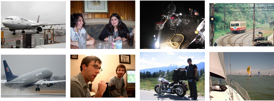
the MATLAB window to run it, and will need to modify it as you go through the session. Part 1: Training and testing an Image Classifier Stage A: Data Preparation The data provided in the directory data consists of images and pre-computed feature vectors for each image. The JPEG images are contained in data/images. The data consists of three image classes (containing aeroplanes, motorbikes or persons) and`background' images (i.e. images that do not contain these three classes). In the data preparation stage, this data is divided as:
The feature vector consists of SIFT features computed on a regular grid across the image (`dense SIFT') and vector quantized into visual words. The frequency of each visual word is then recorded in a histogram for each tile of a spatial tiling as shown. The final feature vector for the image is a concatenation of these histograms. This process is summarized in the figure below: 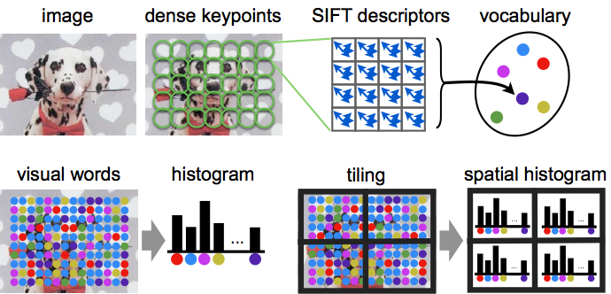
We will start by training a classifier for images that contain aeroplanes. The files data/aeroplane_train.txt and data/aeroplane_val.txt list images that contain aeroplanes. Look through example images of the aeroplane class and the background images by browsing the image files in the data directory. Stage B: Train a classifier for images containing aeroplanes The aeroplane training images will be used as the positives, and the background images as the negatives. The classifier is a linear Support Vector Machine (SVM). Train the classifier by following the steps in exercise1.m. We will first assess qualitatively how well the classifier works by using it to rank all the training images. What do you expect to happen? View the ranked list using the provided function displayRankedImageList as shown in excercise1.m. You can use the function displayRelevantVisualWords to display the image patches that correspond to the visual words which the classifier thinks are most related to the class (see the example embedded in exercise1.m). Stage C: Classify the test images and assess the performance Now apply the learnt classifier to the test images. Again, you can look at the qualitative performance by using the classifier score to rank all the test images. Note the bias term is not needed for this ranking, only the classification vector w. Why? Now we will measure the retrieval performance quantitatively by computing a Precision-Recall curve. Recall the definitions of Precision and Recall: 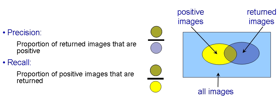 Stage D: Learn a classifier for the other classes and assess its performance Now repeat stages (B) and (C) for each of the other two classes: motorbikes and persons. To do this you can simply rerun exercise1.m after changing the dataset loaded at the beginning in stage (A). Remember to change both the training and test data. In each case record the AP performance measure.
Stage E: Vary the image representation Up to this point, the image feature vector has used spatial tiling. Now, we are going to`turn this off' and see how the performance changes. In this part, the image will simply be represented by a single histogram recording the frequency of visual words (but not taking any account of their image position). This is a bag-of-visual-words representation. A spatial histogram can be converted back to a simple histogram by merging the tiles. Edit exercise1.m to turn the part of the code that does so. Then evaluate the classifier performance on the test images.
Stage F: Vary the classifier Up to this point we have used a linear SVM, treating the histograms representing each image as vectors normalized to a unit Euclidean norm. Now we will use a Hellinger kernel classifier but instead of computing kernel values we will explicitly compute the feature map, so that the classifier remains linear (in the new feature space). The definition of the Hellinger kernel (also known as the Bhattacharyya coefficient) is  where h and h' are normalized histograms. So, in fact, all that is involved in computing the feature map is taking the square root of the histogram values and normalizing the resulting vector to unit Euclidean norm.
Note: when learning the SVM, to save training time we are not changing the C parameter. This parameter influences the generalization error and should be learnt on a validation set when the kernel is changed. Stage G: Vary the number of training images Up to this point we have used all the available training images. Now edit exercise1.m the fraction variable to use 10% and 50% of the training data.
Part 2: Training an Image Classifier for Retrieval using Google images In Part 1 of this practical the training data was provided and all the feature vectors pre-computed. The goal of this second part is to choose the training data yourself in order to optimize the classifier performance. The task is the following: you are given a large corpus of images and asked to retrieve images of a certain class, e.g. containing a bicycle. You then need to obtain training images, e.g. using Google Image Search, in order to train a classifier for images containing bicycles and optimize its retrieval performance. The MATLAB code exercise2.m provides the following functionality: it uses the images in the directory data/myImages and the default negative list data/background_train.txt to train a classifier and rank the test images. To get started, we will train a classifier for horses:
The test data set contains 148 images with horses. Your goal is to train a classifier that can retrieve as many of these as possible in a high ranked position. You can measure your success by how many appear in the first 36 images (this performance measure is `precision at rank-36'). Here are some ways to improve the classifier:
Note: all images are automatically normalized to a standard size, and descriptors are saved for each new image added in the data/cache directory. The test data also contains the category car. Train classifiers for it and compare the difficulty of this and the horse class. Links and further work:
Acknowledgements:
History:
|