Reconnaissance d’objets et vision artificielle 2010/2011Object recognition and computer vision 2010/2011Assignment 2: Stitching photo mosaics
Jean Ponce, Ivan Laptev, Cordelia Schmid and Josef
Sivic
(adapted from A. Efros, CMU, S. Lazebnik, UNC, and A.
Zisserman, Oxford)
Due date: November 2nd 2010
The
goal of the assignment is to automatically stitch images acquired by a
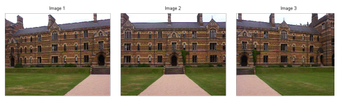
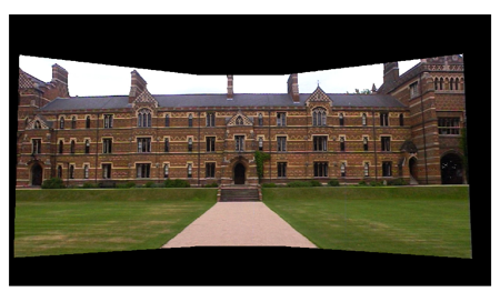
panning camera into a mosaic as illustrated in figures 1 and 2 below.
Fig.1: Three images acquired
by a panning camera.
Fig.2: Images stitched to a
mosaic. Algorithm outline:1. Choose one image as
the reference frame. 2. Estimate homography
between each of the remaining images and the reference image. To estimate
homography between two images use the following procedure: a. Detect local features
in each image. b. Extract feature
descriptor for each feature point. c. Match feature
descriptors between two images. d. Robustly estimate
homography using RANSAC. 3.
Warp each image into the reference frame and composite warped images into a
single mosaic. Tips and detailed description of the algorithm:The
algorithm will be described on the example of stitching images shown in
figure 1. 1. Choosing the reference image. Choosing the middle image of the
sequence as the reference frame is the preferred option, as it will result in
mosaics with less distortion. However, you can choose any image of the
sequence as the reference frame. If you choose image 1 or 3 as the reference
frame, directly estimating homography between images 1 and 3, will be
difficult as they have very small overlap. To deal with this issue, you might
have to “chain” homographies, e.g. H13 = H12 * H23. 2. Estimating homography. a. Detect local features in each image. You can use your feature
detector from assignment 1. Alternatively, you can use function harris.m by A. Efros implementing a simple single scale
Harris corner detector. Note detection of local features with a sub-pixel accuracy is
not required for this assignment. b. Extract feature descriptor for each feature point.
Implement feature descriptor extraction outlined in Section 4 of the
paper “Multi-Image
Matching using Multi-Scale Oriented Patches” by Brown et al. Don’t worry about
rotation-invariance – just extract axis-aligned 8x8 patches. Note
that it’s important to sample these patches from the larger 40x40 window to
have a nice large blurred descriptor. Note, if you
use your multi-scale blob detector from assignmnet 1: As there is almost no
scale change between the supplied images, you can compute descriptors on a
single scale, ignoring the detected characteristic scale associated with each
feature. For example, you can just extract a 40x40 pixel patch around each
detected feature and properly down-sample it to 8x8 pixels to form a
64-dimensional descriptor. For down-sampling, smooth the image with a
Gaussian to remove high spatial frequencies, or use Matlab function “imresize”). You can
also use the more efficient Gaussian pyramid implementation described in the
Brown et al. paper. Don’t
forget to bias/gain-normalize the descriptor. Ignore the Haar wavelet
transform section in the Brown et al. paper. c. Match feature descriptors between two images. Implement
Feature Matching (Section 5 in “Multi-Image
Matching using Multi-Scale Oriented Patches” by Brown et al.). That is, you will need to
find pairs of features that look similar and are thus likely to be in
correspondence. We will call this set of matched features “tentative”
correspondences. You may find function dist2.m useful for distance
computations. For thresholding, use the simpler approach due to Lowe of
thresholding on the ratio between the first and the second nearest neighbors.
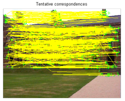
Consult Figure 6b in the paper for picking the threshold. Ignore
Section 6 on fast Wavelet indexing. You can visualize the tentative correspondences
between two images by displaying the feature displacements. For example, to
visualize tentative correspondences between image 1 and 2: (i) show image 1,
(ii) show detected features in image 1 (display only region centers as
points, do not worry about the regions’ scale), (iii) show displacements
between detected features in image 1 and matched features in image 2 by line
segments. This is illustrated in figure 3 and can be achieved using the
following matlab code, where im1_pts and im2_pts are 2-by-n matrices holding (x,y) image locations of
tentatively corresponding features in image 1 and image 2, respectively: figure;
clf; imagesc(im1rgb); hold on; % show
features detected in image 1 plot(im1_pts(1,:),im1_pts(2,:),'+g');
% show
displacements line([im1_pts(1,:);
im2_pts(1,:)],[im1_pts(2,:); im2_pts(2,:)],'color','y') d. Robustly estimate homography using RANSAC. Use a sample of
4-points to compute each homography hypothesis. You will need to write a
function of the form: H
= computeH(im1_pts,im2_pts) where, again, im1_pts and im2_pts are
2-by-n matrices holding the (x,y) locations of n(=4) point correspondences
from the two images and H is the recovered 3x3 homography
matrix. In order to compute the entries in the matrix H, you will
need to set up a linear system of n equations (i.e. a matrix equation of the
form Ah=0 where h is a
vector holding the 8 unknown entries of H). The solution to the
homogeneous least squares system Ax=0
is obtained from the SVD of A by the singular vector corresponding to the
smallest singular value. In Matlab: [U,S,V]=svd(A);
x = V(:,end);
For more details
on homography estimation from point correspondences see a note
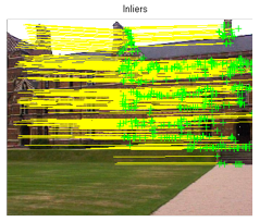
written by David Kriegman. For RANSAC, a very simple implementation performing a
fixed number of sampling iterations is sufficient. You should output a single
transformation that gets the most inliers in the course of all the
iterations. For the various RANSAC parameters (number of iterations, inlier
threshold), play around with a few ``reasonable'' values and pick the ones
that work best. For randomly sampling matches, you can use the Matlab randperm function. You should
display the set of inliers as illustrated in figure 3. Finally,
after you find the set of inliers using RANSAC, don’t forget to re-estimate
the homography from all inliers. 3. Warping and compositing. Warp each image into the reference frame
using the estimated homography and composite warped images into a single
mosaic. You can use the vgg_warp_H function
for warping. Here is an example code to warp and composite images 1 and 2 : First, define a mosaic image to warp all the images onto.
Here we assume image 2 as the reference image, and map this image to the
origin of the mosaic image using the identity homography (eye(3) in Matlab). bbox =
[-400 1200 -200 700] % image space for mosaic Im2w =
vgg_warp_H(Im2, eye(3), ’linear’, bbox); % warp image 1 to mosaic image Now warp image 1 to a separate mosaic image using
estimated homography H12 between image 1 and image 2 Im1w =
vgg_warp_H(Im1, H12, ’linear’, bbox); and finally combine the mosaic images by taking the pixel
with maximum value from each image. This tends to produce less artifacts than
taking the average of warped images. imagesc(double(max(Im1w,Im2w))/255); |
|
|