Reconnaissance d’objets et vision artificielle 2010/2011
Object recognition and computer vision 2010/2011
Assignment 1: Scale-invariant blob detection
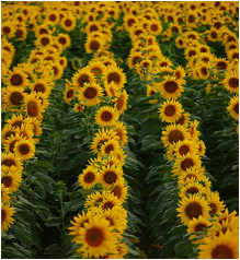 
Left:
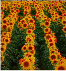
Example input image. Right: Scale-invariant blob detections overlaid.
Jean Ponce, Ivan Laptev, Cordelia Schmid and Josef
Sivic
(adapted from Svetlana Lazebnik, UNC)
Due date: October 19th 2010
The
goal of the assignment is to implement a Laplacian blob detector as discussed
in the lectures. An example of scale-invariant blob detection is shown above.
Algorithm outline:
1.
Build a Laplacian scale space, starting with some initial scale and going for
n iterations:
1. Generate a scale-normalized Laplacian of Gaussian filter at a given
scale “sigma”.
1. Filter image with the scale-normalized Laplacian.
2. Save square of Laplacian filter response for current level of scale
space.
3. Increase scale by a factor k.
2.
Perform non-maximum suppression in scale space.
3.
Display resulting circles at their characteristic scales.
Tips
· You
have to choose the initial scale, the factor k by which the scale is
multiplied each time, and the number of levels in the scale space. Reasonable
value for the initial scale is sigma=2 pixels, using 10 to 15 levels for the
scale pyramid. The multiplication factor should depend on the largest scale at
which you want regions to be detected (try e.g. k=2^(0.25)).
· You can use the Matlab
function fspecial
for generating the scale-normalized Laplacian of Gaussian filter at a given
scale “sigma”:
filt_size
= 2*ceil(3*sigma)+1; % filter
size
LoG = sigma^2 * fspecial('log', filt_size,
sigma);
· You can use the Matlab function imfilter to convolve the image with
the filter, e.g.:
imFiltered
= imfilter(im, LoG, 'same', 'replicate');
· You
may want to use a three-dimensional array to represent your scale space. It
would be declared as follows:
scale_space = zeros(h,w,n); % [h,w] - dimensions of
image, n - number of levels in scale space
Then scale_space(:,:,i) would give you the i-th level of the scale space. Alternatively, if
you are storing different levels of the scale pyramid at different
resolutions, you may want to use a cell array, where each "slot"
can accommodate a different data type or a matrix of different dimensions.
Here is how you would use it:
scale_space = cell(n,1); %creates a cell array with n
"slots"
scale_space{i} = my_matrix; % store a matrix at
level i
· On the non-maximum suppression in
scale space. The goal is to find pixels, which are local maxima in the scale-space.
This amounts to finding pixels with the filter response (strictly) greater
than its 26 (3x3x3 neighbourhood) scale-space neighbours, considering also
the adjacent scales as illustrated in figure 2 of David Lowe's paper.
· To
perform non-maximum suppression in scale space, you may first want to do
non-maximum suppression in each 2D slice separately. For this, you may find
functions nlfilter, colfilt or ordfilt2 useful. To extract the final
nonzero values (corresponding to detected regions), you may want to use the find function.
· You
also have to set a threshold on the squared Laplacian response above which to
report region detections. A reasonable value is 0.001, but you should play
around with different values and choose one you like best.
· To
display the detected regions as circles, you can use this function (or feel free to write your own).
Don't forget that there is a multiplication factor that relates the scale at
which a region is detected to the radius of the circle that most closely
"approximates" the region.
· If you
decide to experiment with different implementation choices for building the
scale space and nonmaximum suppression, you may want to compare these choices
according to their computational efficiency. To time different routines, use tic and toc commands.
· Apply
the detector to greyscale versions of colour images. In Matlab, you can
convert a color image to greyscale using
Im_gray = mean(Im_rgb,3);
Make sure the image values are scaled between 0 and 1.
· If you are new to
MATLAB, have a look at the very useful tutorials
(from Martial Hebert at
CMU). They will give you overview of basic necessary functions: basic operations, programming, working with images.
· You may also want check
this code for an example of a Harris interest point detector: Sample Harris detector code.
Test images
Here
are four images to test your code. Also
run your code on two images of your own choice.
What to hand in
· You
should implement the Laplacian blob detector as described in the algorithm
outline above.
· Motivated students can also implement the efficient difference of
Gaussian approximation described in section 3 of David Lowe’s paper.
However, this is not required and will not be marked.
You
should prepare a (very brief) report including the following:
· A figure showing the 2D Laplacian of Gaussian filter
(use Matlab functions surf(LoG)
or mesh(LoG) to visualize the filter).
· Short answers to the following two questions: (i) What
does it mean when a filter is separable? (ii) Is the Laplacian of Gaussian
filter separable?
· For image “sunflowers.jpg” show the squared
Laplacian response for three different scales (sigma=2, 4 and 8 pixels).
· Show a graph of the Laplacian response across
scales, i.e. the scale “sigma” on the x-axis and the squared Laplacian filter
response on the y-axis, for two image points corresponding to: (i) the large
sunflower in the foreground (image coordinates from top-left corner [row=327,
column=128] and (ii) the small sunflower in the background (image coordinates
[row=62, column=130]). On which scale is the strongest response for the two
points?
· Show the output of your detector (i.e. detected regions shown as circles of
different sizes overlaid over the image) on all test images.
Instructions for formatting and handing-in assignments:
· At the top of the first page of
your report include (i) your name, (ii) date, (iii) the assignment number and
(iv) the assignment title.
· The report should be a single pdf
file and should be named using the following format:
A#_lastname_firstname.pdf, where
you replace # with the assignment number and “firstname” and
“lastname” with your name, e.g. A1_Sivic_Josef.pdf.
· Zip your code and any additional files (e.g.
additional images) into a single zip file using the same naming convention as
above, e.g. A1_Sivic_Josef.zip. We do not intend to run your code, but we may look at it and try to
run it if your results look wrong.
Send
your report, code, and your two additional test images to Josef Sivic <Josef.Sivic@ens.fr>.
Helpful resources
· Useful Matlab tutorials (from Martial
Hebert at CMU): basic operations, programming, working with images.
· Sample Harris detector code.
· Nice Slides
by Svetlana Lazebnik on feature detection describing also scale invariant
blob detection (slides 32—49).
· Blob detection on
Wikipedia.
· D.
Lowe, "Distinctive
image features from scale-invariant keypoints," International
Journal of Computer Vision, 60 (2), pp. 91-110, 2004. This paper contains
details about efficient implementation of a Difference-of-Gaussians scale
space.
· T. Lindeberg, "Feature
detection with automatic scale selection," International Journal of
Computer Vision 30 (2), pp. 77-116, 1998. This is somewhat advanced reading
for those of you who are really
interested in the gory mathematical details.
|