Reconnaissance d’objets et vision artificielle 2009/2010

Object recognition and computer vision 2009/2010

Image source: Antonio Torralba

Final project

Jean Ponce, Ivan Laptev, Cordelia Schmid and Josef Sivic

Due date: December 20th 2009

The goal of the final project is to implement and improve an algorithm for (1) image classification OR (2) object detection/localization.
You will evaluate the performance of the algorithm on state-of-the-art image datasets. You will build on assignments you completed during the course.

You are encouraged to work alone but you can also form groups of two or three people. Each group will submit a single final report. Details of the report requirements are given below.

Each group should choose one of the two proposed projects. You can propose your own alternative project, but you need to validate your project with the course instructors:
please email or come to discuss in person with either Ivan Laptev <Ivan.Laptev@ens.fr> or Josef Sivic <Josef.Sivic@ens.fr>.

Quick links to instructions for:

1. Project 1: Image classification
2. Project 2: Object detection/localization
3. Writing and submitting your final project report
   

---

Project 1 - Image Classification

The Data (46 MB, 3,487 images, 100 object classes) the source: Caltech Vision Group

The goal is to implement and evaluate an advanced system for bag-of-features image classification. The task is to perform a 100-class image classification on the challenging dataset of 100 object
classes.


Experimental setup

Most the 100 object classes have a total of 35 images. A small number of object classes have less than 35 available images. You should use the first 15 images from each class for training and the remaining up to 20 images for testing. Perform multi-way classification, i.e. assign each test image to one of the 100 classes. For each class compute the accuracy, i.e. the percentage of correctly classified test images. As a single number measure of recognition performance of your system average the accuracy across all 100 classes.


Outline of the project

As a baseline, run your image classification system from Assignment 3 (bag-of-features representation with the nearest neighbor classifier).
For computing the visual dictionary randomly sample a 100,000-200,000 descriptors from all training images.

Next, the goal is to improve recognition performance of this baseline system.
Below are suggested extensions.

The goal of this project is to implement a variant of Histograms of Oriented Gradients (HOG) object detector by Dalal & Triggs [CVPR05] and to evaluate it on a difficult state-of-the-art dataset. The three main steps of this project are (i) implementation of HOG image descriptor, (ii) learning linear SVM object detector using “hard negatives” and (iii) evaluation of object detector on the PASCAL VOC 2007 dataset.

Data and code for download

• Pascal VOC 2007 Training and validation data (450MB tar file)
• VOC development code and documentation
• A few useful Matlab functions (NEW)
  
• Alternative SVM packages with interface to Matlab:
  
  SVM-light (recommended)
  LibSVM
  STPRTool
  
  (In most cases these packages should work directly on your Windows/Linux systems. In some cases, however, you may need to compile them, see instructions inside packages in this case)

Task description

1.      Histograms of Oriented Gradients (HOG). HOG is one of the most successful recent object descriptors. You should implement a variant of HOG either as described in the original paper by Dalal & Triggs [CVPR05] or as described in the following (a simplified version). To compute HOG descriptor for an image patch:  

(a) subdivide the patch into a grid of equal spatial cells (nx,ny),
(b) for each cell compute a histogram of gradient orientations descretized into n orientations bins. Gradient orientation should be computed at every pixel as atan(Ix/Iy) where Ix and Iy are image derivatives. You can efficiently compute image derivatives by convolution with the filter of the form [-1 0 1] for Ix or [-1 0 1]^T for Iy.  A histogram should be accumulated from gradients at all pixels inside the cell. When accumulating the histogram, the contributions of different pixels should be weighted proportionally to the value of the pixel gradient magnitude sqrt(Ix^2+Iy^2).
(c) concatenate histograms of all cells and normalize resulting descriptor vector w.r.t. its l2-norm.
 
To run object detection you will need to compute and classify HOG descriptors for a very large number of image windows. Your HOG implementation therefore should be efficient. HOG can be computed efficiently using integral gradient images, which are analogous to the standard integral image discussed in lecture 6 (slides 34-47) in the context of face detection.  You will compute n integral images, one for each discretized gradient orientation bin. The computation proceeds as follows: (i) pre-compute and discretize gradient orientations for the whole image, (ii) compute orientation layers  I1…n such that Ij has values 1 for all image pixels with gradient orientation j and zeros otherwise (I1…n should have the same size as the input image I). Multiply each layer I1…n by the gradient magnitude, i.e. in Matlab notation Ij_weighted=Ij.*Igradmag; where Igradmag= sqrt(Ix.^2+Iy.^2);. Integrate each layer along x and y dimensions as Ij_weighted_integral=cumsum(cumsum(Ij_weighted,1),2).

Integral gradient image computed above enables to obtain a histogram of gradient orientations for any image rectangle efficiently in constant time.  Given rectangular image patch represented by points (p11,p12,p22,p21), the histogram of its gradient orientations H=h1…n can be computed in terms of its individual bins as hj=Ij_weighted_integral(p22)- Ij_weighted_integral(p12)- Ij_weighted_integral(p21)+ Ij_weighted_integral(p11). (For the related explanation and use of integral images see Section 2 of Viola & Jones IJCV 2004 paper.) You can now efficiently compute gradient histograms for all cells of a HOG descriptor; concatenate histograms into a descriptor vector and normalize. Concerning what HOG parameter values to use, n=8 and and nx=10, ny=6 can be recommended for object classes “motorbike” and “horse” that will be considered below.

In summary, you should implement two Matlab functions with the following interfaces:

ghistintegral=gradimageintegral(img,qnum);

%

% gradimageintegral: computes gradient integral image

% Input  img: original gray-value image of size [ysz,xsz]

%        qnum: number of gradient orientations (default 8)

% Output ghistintegral: integral gradient image of

%        dimension [ysz,xsz,qnum]

%

hog=hogintegral(ghistintegral,bbox,nx,ny);

%

% hogintegral: computes HOG descriptors for given image windows

% Input  ghistintegral: integral gradient image

%        bbox: image window(s) represented as [x1 y1 x2 y2; ...]

%        nx,ny: number of (equal-size) descriptor cells along x and y window dimensions

%       

The following test should be used to validate your HOG implementation. In the first image (get image here) mark a car wheel and compute HOG descriptor for the corresponding image patch (use HOG parameters n=4, nx=4, ny=4). In the second image (get image here) compute HOG descriptors for image windows at all possible image locations, compute corresponding HOG descriptors and evaluate the Euclidean distance between all HOGs in the second image to the selected HOG descriptor in the first image. Display matching windows that minimize HOG distance. You should obtain a similar result as below. Computing integral images, extracting HOG descriptors and matching for this example should not take more than a few seconds.

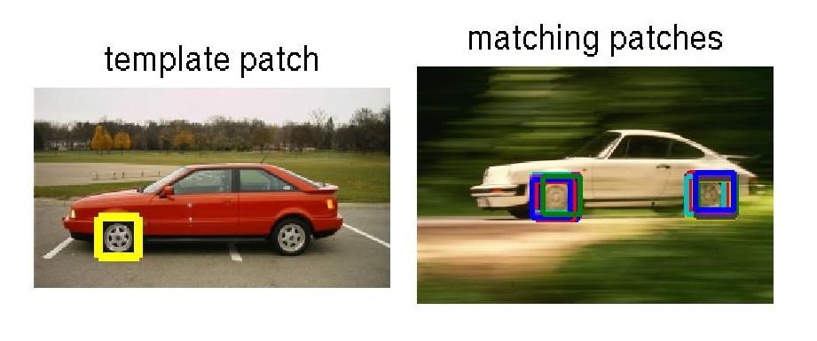Figure 1. Matching HOG descriptors between two images. Left: The template patch. Right: The top matching patches in another image overlaid.

2.      Training object detector. In this part of the project you should learn a linear SVM object classifier, similar as you have done in Assignment 4.  Differently to Assignemts 4, here, you will have to (i) collect positive and negative training samples from annotated training images and (ii) describe each sample with a HOG descriptor. Training samples should be collected from the “train” subset of PASCAL VOC 2007 dataset (450Mb). Download the dataset together with the VOC development kit, install the kit and edit VOCopts.datadir variable in VOCinit.m to point to your VOCdata folder. Run VOCinit.m to initialize VOCopts variable. To collect HOG descriptors for positive training samples you can use the following function getpossamples.m To collect training samples of the “motorbike” class you can run this function with the following arguments:

possamples=getpossamples(VOCopts,’motorbike’,’train’,8,10,6);

You will need to implement a function ‘gradimageintegral’ for computing gradient integral images as well as the function ‘hogintegral’ for computing HOG descriptors before using getpossamples.m. Once you obtain positive training samples, you should collect negative training samples from e.g. 2000 random windows of training images which do not overlap with positive samples. Train a liner SVM and obtain a classification hyperplane as previously done in Assignment 4. Validate your classifier on positive and negative samples of the validation set. To obtain positive samples of the validation use command: possamples=getpossamples(VOCopts,’motorbike’,’val’,0.1,8,0,10,6,inf); Negative samples for the validation set should be obtained by a similar procedure as used to collect negative samples for the training set. Evaluate performance of the classifier on the validation set by computing ROC curve and Area Under the Curve (AUC) using roc.m

Good negative samples are important for training a good classifier. The technique known as bootstrapping selects “hard negative” samples for the next round of training by running the current classifier on negative images and collecting high-confident responses. Use bootstrapping to collect hard negative samples (e.g. 2000) from the negative images in the training set and then re-train a classifier using original positive and original+new negative samples. Evaluate performance of the new classifier in terms of ROC and AUC on exactly the same validation samples as before and compare results to the ones obtained in the first training round. You should see an improvement. Although the first round of bootstrapping maybe sufficient, you may apply bootstrapping further by iteratively collecting new hard negative samples and re-training your classifier.

Train classifiers according to the above scheme for at least two object classes, e.g. ‘motorbike’ and ‘horse’.

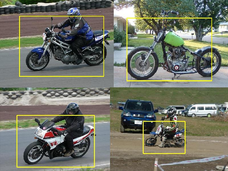
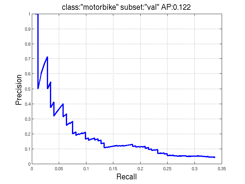
3.      Detection and evaluation. Similar to Assignment 4 you should run window-scanning method to detect instances of target object classes. To merge multiple detections you should apply Non-maxima suppression developed in Assignment 4. To detect objects with different sizes and positions in the image, here you should examine image windows with all locations and sizes (your spatial window step size can increase for large windows, a reasonable scale step is a factor 2^0.25). You can easily extract a HOG descriptor at any image location and window size by providing different input bounding boxe to your hogintegral function. You should apply your detection algorithm to all 2510 images in the validation set. If you experience difficulties in processing this number of images, you can simplify the problem and reduce validation set to its subset with images containing instances of the target class, for example 125 motorbike images and 148 horse images. You should finally evaluate detection results using Precision-recall and Average Precision (AP). Use function VOCevaldet.m (provided in VOC development kit) for this purpose. You are expected to get results similar to the one below. Evaluate detection on at least two object classes (e.g. 'motorbike' and 'horse') and show a few examples of high-confident correct detections (True Positives), high-confident false detections (False Positives) and non-detected positive instances (True Negatives).

4.      Improve detections with non-linear SVM (optional):  You can improve your detector by training a non-linear SVM and use it to filter initial detections returned by the linear SVM classifier.

You should describe and when possible illustrate the following in your final report:

1.      Describe your implementation of HOG features and illustrate the matching of HOG descriptors on the two provided example car images.  Discuss and motivate the need of normalization of HOG descriptor.

2.      Demonstrate results of validating learned classifiers on the validation set in terms of ROC and AUC. Demonstrate the effect of bootstrapping (for groups of 2 or 3 people).

3.      Report object class detection results on the validation set for your chosen set of classes. Illustrate and discuss high-confident True Positives and False Negatives as well as True Negatives (i.e. missed detections).

4.      (Optional) report detection improvement in terms of PR-curves and AP using non-linear SVM classifier.

5.    See instructions for writing and submitting the final project report.

References

[1] N. Dalal and B. Triggs, Histograms of Oriented Gradients for Human Detection, CVPR 2009 (PDF)
[2] Robust Real-Time Object Detection, IJCV 2004 (PDF)
[3] PASCAL VOC 2007 Challenge (Workshop slides in PDF)

Instructions for writing and submitting the final project report

• For the final project, you do not need to hand-in any code. Only hand-in a 3 page report in the format of the submission to the IEEE Computer Vision and Pattern Recognition conference (CVPR) . Use the latex or word templates provided at the CVPR Author Guidelines webpage. Note, that your are asked to produce only a 3-page double-column report (in contrast, a standard CVPR submission is up-to 8 pages).