Reconnaissance d’objets et vision artificielle 2009/2010
Object recognition and computer vision 2009/2010

Assignment 4: Simple Face Detector

Jean Ponce, Ivan Laptev, Cordelia Schmid and Josef Sivic

Due date: December 8th 2009

The goal of this assignment is to implement a simple face detector. You will experiment with the so-called “window-scanning” method by implementing its main steps and analyzing detection performance on real images. We will consider a rather simple implementation of the detector to (a) have a better overview of the method and (b) to understand the need of more sophisticated detection tools for achieving better performance. An extended and better performing version of object detection will be considered in the final assignment of this course.

Data and code for download

• Training and test images
• Alternative SVM packages with interface to Matlab
  SVM-light (recommended)
  LibSVM
  STPRTool
  (In most cases these packages should work directly on your Windows/Linux systems. In some cases, however, you may need to compile them, see instructions inside packages in this case)

Task description

1. Normalize training images: load positive and negative training images from images/possamples.mat and images/negsamples.mat respectively. These are 24x24 pixel grey-scale image patches with cropped faces and non-faces concatenated along the 3^rd array dimension. To reduce effect of light variation, write a function to normalize input pixels of each individual patch to the mean value 0 and standard deviation 1.

2. Train linear SVM: for a subset of 1000 positive and 1000 negative normalized patches train a linear SVM model using e.g. <svmlearn> function of SVM-light package (hint: use matlab command <reshape> to transform 3D array with N image patches to 2D array with N columns representing pixel values of patches stacked into vectors).

a. Validate recognition accuracy on a separate validation set of 1000 positive and 1000 negative normalized patches using <svmclassify> function of SVM-light

b. Analyze and report accuracies for different values of C-parameter of SVM, choose the best C (hint: try small C-values in the range 0.1- 0.0001)

c. Reconstruct decision hyper-plane W from support vectors and implement your own linear classifier of the form confidence=W*X+b Make sure that your classifier confidence>0 gives exactly the same result as <svmclassify> (hint: for SVM-light package you will find values alpha_i * y_i for training samples x_i stored in model.a(i), parameter b is saved in model.b)

d. “Reshape-back” the hyperplane W into a 24x24 patch, display it with <imagesc> (you should see something meaningful!), include the plot into your report and discuss it

e. Re-train linear SVM classifier using all available training samples and the best found C-value.

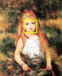
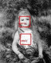
3. Scanning-window detection: implement a function that for a given image (i) generates bounding boxes of size 24x24 pixels for all valid positions (ii) crops an image into overlapping 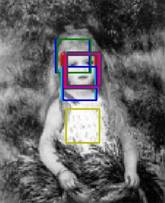patches according to all bounding boxes; (iii) normalizes all patches separately as done for training images in Step 1 above (iv) classifies all patches using linear SVM model trained in Step 2-e above; (v) returns bounding boxes, corresponding normalized patches and confidence scores for all high-confident detections. Apply your window-scanning function to jpeg test images in images/ folder and display original images + rectangles corresponding to high confident detections (i.e. conf>0). Include images with detections in your report (hint1: use your own classifier of the form conf=W*X+b as it tends to be much faster compared to <svmclassify> function of SVM-light; hint2: use matlab function rectangle(‘Position’,[x y width height]) to plot rectangles on top of the image). Example result of what you should expect to get at this step is illustrated on the right.

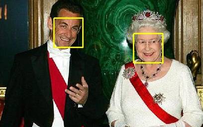
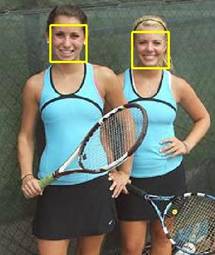
4. Non-maximum suppression: write a function that merges multiple detections with similar coordinates. For this you can follow agglomerative clustering algorithm as follows: (i) choose bounding box D corresponding to the most confident detection in the list, (ii) find all detections with sufficient overlap to D, (iii) average selected detections into one bounding box and assign its confidence by the confidence of D, (iv) remove merged detections from the list and continue with Steps (i)-(iii) until all detections are merged. Manually find a suitable confidence threshold and display obtained detection with confidence>threshold using the same threshold for all images, include plots into your report, discuss correct detections and failure cases. (hint: to measure overlap between two bounding boxes A,B use ratio IntersectionArea(A,B)/UnionArea(A,B)) Example result of what you should expect to get at this step is illustrated on the right.

5. Improve detections with non-linear SVM (optional): As you may have noticed, the developed linear SVM detector is not perfect. A simple way to improve the detector performance is to apply a more costly and sophisticated classifier to the set of initial detections. Train a non-linear SVM classifier with RBF kernel using the same training data as in Step 2-e above. Try SVM RBF parameter gamma=0.002 and C=10. Non-linear SVM is rather slow to evaluate on all image windows. Instead, apply it to the initially detected patches in Step 3 followed by the non-maximum suppression in Step 4. You should see improved detection results. (Note: you cannot use a linear classifier function conf=W*X+b in the case of non-linear SVM).

What to hand in

You should hand in your code together with a brief report illustrating the steps of your experiments:

1. Accuracy values on the validation set when training linear SVM for different C-values in Step 1-b

2. Visualization of the linear hyperplane W in Step 2-d

3. High-confident scanning-window detections on test images in Step 3

4. Results of non-maximum suppression applied to detections on test images in Step 4 + discussion of results

5. (Optional) improved detection results using non-linear classifier.

Instructions for formatting and handing-in assignments:

• At the top of the first page of your report include (i) your name, (ii) date, (iii) the assignment number and (iv) the assignment title.
• The report should be a single pdf file and should be named using the following format: A#_lastname_firstname.pdf, where you replace # with the assignment number and “firstname” and “lastname” with your name, e.g. A4_Laptev_Ivan.pdf.
• Zip your code into a single zip file using the same naming convention as above, e.g. A4_Laptev_Ivan.zip. We do not intend to run your code, but we may look at it and try to run it if your results look wrong.

Send the pdf file of your report and the zipped code in two separate files to Ivan Laptev <Ivan.Laptev@ens.fr>