Release 2013A
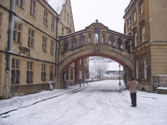
The goal of instance-level recognition is to match (recognize) a specific object or scene. Examples include recognizing a specific building, such as Notre Dame, or a specific painting, such as `Starry Night’ by Van Gogh. The object is recognized despite changes in scale, camera viewpoint, illumination conditions and partial occlusion. An important application is image retrieval - starting from an image of an object of interest (the query), search through an image dataset to obtain (or retrieve) those images that contain the target object. The goal of this session is to get basic practical experience with the methods that enable specific object recognition. It includes: (i) using SIFT features to obtain sparse matches between two images; (ii) using affine co-variant detectors to cover changes in viewpoint; (iii) vector quantizing the SIFT descriptors into visual words to enable large scale retrieval; and (iv) constructing and using an image retrieval system to identify objects. Getting startedRead and understand the requirements and installation instructions. The download links for this practical are:
After the installation is complete, open and edit the script exercise1.m in the MATLAB editor. The script contains commented code and a description for all steps of this exercise, relative to Part I of this document. You can cut and paste this code into the MATLAB window to run it, and will need to modify it as you go through the session. Other files exercise2.m, exercise3.m, and exercise4.m are given for Part II, III, and IV.Note: the student packages contain only the code required to run the practical. The complete package, including code to preprocess the data, is available on GitHub.
Part I: Sparse features for matching specific objects in imagesStage I.A: SIFT features detectorThe SIFT feature has both a detector and a descriptor. We will start by computing and visualizing the SIFT feature detections for two images of the same object (a building facade). Load an image, rotate and scale it, and then display the original and transformed pair: % Load an imageim1 = imread('data/oxbuild_lite/all_souls_000002.jpg') ;% Let the second image be a rotated and scaled version of the firstim3 = imresize(imrotate(im1,35,'bilinear'),0.7) ;% Display the imagessubplot(1,2,1) ; imagesc(im1) ; axis equal off ; hold on ;subplot(1,2,2) ; imagesc(im3) ; axis equal off ;A SIFT frame is a circle with an orientation and is specified by four parameters: the center tx, ty, the scale s, and the rotation θ (in radians), resulting in a vector of four parameters (s, θ, tx, ty). Now compute and visualise the SIFT feature detections (frames): % Compute SIFT features for each[frames1, descrs1] = getFeatures(im1, 'peakThreshold', 0.01) ;[frames3, descrs3] = getFeatures(im3, 'peakThreshold', 0.01) ;subplot(1,2,1) ; imagesc(im1) ; axis equal off ; hold on ;vl_plotframe(frames1, 'linewidth', 2) ;subplot(1,2,2) ; imagesc(im3) ; axis equal off ; hold on ;vl_plotframe(frames3, 'linewidth', 2) ;Examine the second image and its rotated and scaled version and convince yourself that the detections overlap the same scene regions (even though the circles have moved their image position and changed radius). It is helpful to zoom into a smaller image area using the MATLAB magnifying glass tool. This demonstrates that the detection process transforms (is co-variant) with translations, rotations and isotropic scalings. This class of transformations is known as a similarity or equiform.
Now repeat the exercise with a pair of natural images. Start by loading the second one: % Load a second imageim2 = imread('data/oxbuild_lite/all_souls_000015.jpg') ;and plot images and feature frames. Again you should see that many of the detections overlap the same scene region. Note that, while repeatability occurs for the pair of natural views, it is much better for the synthetically rotated pair.
Stage I.B: SIFT features descriptors and matching between imagesNext we will use the descriptor computed over each detection to match the detections between images. We will start with the simplest matching scheme (first nearest neighbour of descriptors) and then add more sophisticated methods to eliminate any mismatches.
Hint. You can visualize a subset of the matches using: figure; plotMatches(im1,im2,frames1,frames2,matches(:,3:200:end));Stage I.C: Improving SIFT matching using Lowe’s second nearest neighbour testLowe introduced a second nearest neighbour (2nd NN) test to identify, and hence remove, ambiguous matches. The idea is to identify distinctive matches by a threshold on the ratio of first to second NN distances. In the MATLAB file, the ratio is
Stage I.D: Improving SIFT matching using a geometric transformationIn addition to the 2nd NN test, we can also require consistency between the matches and a geometric transformation between the images. For the moment we will look for matches that are consistent with a similarity transformation which consists of a rotation by θ, an isotropic scaling (i.e. same in all directions) by s, and a translation by a vector (tx, ty). This transformation is specified by four parameters (s,θ,tx, ty) and can be computed from a single correspondence between SIFT detections in each image.
Hint. Recall from Stage I.A that a SIFT feature frame is an oriented circle and map one onto the other. The matches consistent with a similarity can then be found using a RANSAC inspired algorithm, implemented by the function RANSAC-like algorithm for geometric verification
After this algorithm the inliers are consistent with the transformation and are retained, and most mismatches should now be removed.
If more matches are required the geometric transformation can be used alone, without also requiring the 2nd NN test. Indeed, since the 1st NN may not be the correct match, a list of potential (putative) matches can be generated for each SIFT descriptor by including the 1st NN, 2nd NN, 3rd NN etc. Investigate how the number of correct matches (and time for computation) grows as the potential match list is extended, and the geometric transformation is used to select inliers. To this end:
Hint. You can use MATLAB’s tic ; pause(3) ; tocwill pause MATLAB for three seconds and return an elapsed time approximately equal to 3. See In this case, there is foreshortening (anisotropic scaling) and perspective distortions between the images (as well as in-plane rotation, translation and scaling). A circle in one image cannot cover the same scene area as a circle in the other, but an ellipse can. Affine co-variant detectors are designed to find such regions. In the following we will compare the number of matches using a similarity and affine co-variant detector as the viewpoint becomes progressively more extreme. The detectors are SIFT (for similarity) and SIFT+affine adaptation (for affine), while the descriptor are in both cases SIFT.
Note. There are many other detector variants that could be used for this task. These can be activated by the method option of
getFeatures.m (see also help vl_covdet).Part III: Towards large scale retrievalIn large scale retrieval the goal is to match a query image to a large database of images (for example the WWW or Wikipedia). The quality of a match is measured as the number of geometrically verified feature correspondences between the query and a database image. While the techniques discussed in Part I and II are sufficient to do this, in practice they require too much memory to store the SIFT descriptors for all the detections in all the database images. We explore next two key ideas: one to reduce the memory footprint and pre-compute descriptor matches; the other to speed up image retrieval.
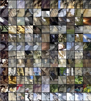
Stage III.A: Accelerating descriptor matching with visual wordsInstead of matching feature descriptors directly as done in Part I and II, descriptors are usually mapped first to discrete symbols, also called visual words, by means of a clustering technique like K-Means. The descriptors that are assigned to the same visual word are considered matched. Each of the rows in the following figure illustrates image patches that are mapped to the same visual word, and are hence indistinguishable by the representation.
Then, matching two sets of feature descriptors (from two images) reduces to finding the intersection of two sets of symbols.
[Skip to Stage III.B on fast track] Often multiple feature occurrences are mapped to the same visual word. In this case
Stage III.B: Searching with an inverted indexWhile matching with visual words is much faster than doing so by comparing feature descriptors directly, scoring images directly based on the number of geometrically verified matches still entails fitting a geometric model, a relatively slow operation. Rather than scoring all the images in the database in this way, we are going to use an approximation and count the number of visual words shared between two images. To this end, one computes a histogram of the visual words in a query image and for each of the database images. Then the number of visual words in common can be computed from the intersection of the two histograms. The histogram intersection can be thought as a similarity measure between two histograms. In practice, this measure can be refined in several ways:
Computing histogram similarities can be implemented extremely efficiently using an inverted file index. In this exercise, inner products between normalized histograms are computed quite efficiently using MATLAB's built-in sparse matrix engine. We now apply this retrieval method to search using a query image within a 660 image subset of the Oxford 5k building image set.
Stage III.C: Geometric rescoringHistogram-based retrieval results are good but far from perfect. Given a short list of top ranked images from the previous step, we are now going to re-score them based on the number of inlier matches after a geometric verification step.
Stage III.D: Full systemNow try the full system to retrieve matches to an unseen query image.
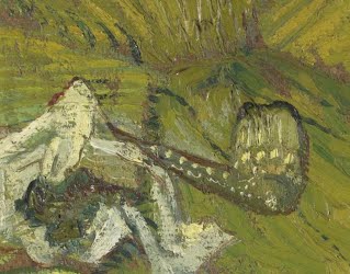
Part IV: Large scale retrieval[Skip and end here on fast track] The images below are all details of paintings. The goal of this last part of the practical is to identify the paintings that they came from. For this we selected a set of 1734 images of paintings from Wikipedia.
We follow route (3) here. Look through and run Note, although the index is stored locally, the matching images are downloaded from Wikipedia and displayed. Click on the image to reach the Wikipedia page for that painting (and hence identify it).
Take note of the code output:
That completes this practical. Links and further work
Acknowledgements
|

 Notice that there are many mismatches.


Texte d'origine
Proposer une meilleure traduction